
TESTING THE SOLOW HYPOTHESIS FOR FISCAL CONVERGENCE: A DYNAMIC SPATIAL ANALYSIS
Ömer Tarık GENÇOSMANOĞLU
 *
*
Kemal Buğra YAMANOĞLU
*
Abstract. The study of regional fiscal convergence is a recent extension of the neoclassical growth theory. Various studies have shown the existence of fiscal convergence across countries or states in federally governed countries. This paper tests the growth theory on income and fiscal variables differently in a centrally ruled country. Therefore, we estimate spatial and non-spatial panel models from 2004 to 2022 for Türkiye. A general-to-specific methodology is applied for selecting an appropriate model to determine spatial interactions of the variables by using the panel data at the level of 81 Turkish provinces. The Ordinary Least Squares (OLS) estimation results from the non-spatial model partially validate the growth theory as the study does not find evidence of absolute convergence for government expenditures. The results, however, confirm the conditional convergence for all variables. The Maximum Likelihood (ML) method is applied for the estimation of the dynamic and static spatial panel models to explain their spatial interactions. The ML findings are consistent with the OLS results. Moreover, unlike direct and total effects, it is not possible to define indirect effects explaining spatial spillover effects in the short and long terms.
Key words: spatial econometrics, dynamic spatial panel models, income convergence, fiscal convergence.
1. INTRODUCTION
The convergence phenomenon predicted by the neoclassical (Solow) growth theory has, on the one hand, mostly been linked to income and numerous studies have been undertaken. On the other, there has been growing research into whether the convergence hypothesis holds for other macroeconomic variables such as public spending, taxes, imports, or exports. One of the primary reasons for this is that governments are increasingly pursuing fiscal policies that try to eliminate disparities in growth and development between countries or across regions.
A large portion of the relevant research conducted in this context has focused on the convergence of fiscal variables, particularly tax revenues and public spending. The Solow growth model implies that tax revenues are a constant proportion of total income and public expenditures should be equal to tax revenues under the balanced budget condition. As a consequence, we expect fiscal variables to grow at the same rate as total income. In other words, the convergence in fiscal variables should follow a parallel course to income. A mathematical derivation of this proposition was provided by Yamanoğlu (2022).
The existing literature, although empirically demonstrating convergence in fiscal variables, has nevertheless been limited to considering the incidence of convergence across countries or states in federally administered countries (Scully, 1991; Sanz and Velazquez, 2001; Annala, 2003; Gemmell and Kneller, 2003; Coughlin et al., 2007; Perovic et al., 2016; Acemoğlu and Molina, 2021; Kremer et al., 2021). To put it another way, Solow’s theory of fiscal variables has yet to be proven in centrally governed economies. Additionally, the related research, which commonly employs cross-sectional or panel methodologies, has barely included analyses of spatial interactions between states or nations (Annala, 2003; Perovic et al., 2016).
In reality, a country’s political and administrative structures inevitably influence its public finances. For example, in countries with centralised administration, the main concerns of the governments are to eliminate income inequalities and gaps in economic development levels between regions, as well as to ensure a fair distribution of resources and public services throughout the country. Political considerations have also more or less influence on the budget and fiscal policies implemented to achieve their goals. Therefore, governments may implement policies that favour specific groups or regions when planning public expenditures. In summary, countries with central governments might differ from those governed by the federal system concerning public finance.
The purpose of this paper is to test Solow’s theory on fiscal variables in a centrally ruled country, namely Türkiye. The insights from the Turkish example could allow us to assess the outcomes of other research investigating federal systems. This study, therefore, makes several important contributions to the existing literature. First, the fiscal convergence proposition based on the growth theory is tested for a country ruled by a central government for the first time through the example of Türkiye. The study explores the presence of fiscal convergence in relation to income levels and provides helpful understanding by demonstrating different convergence patterns. Second, this is one of the rare studies that uses the dynamic and static spatial models together in fiscal convergence analysis. Studies have also scarcely applied the dynamic spatial analysis for income convergence for Türkiye. Third, the spatial spillover effects of fiscal variables are assessed in comparison with income. The results show no evidence of absolute convergence for government expenditures, although all three variables converge conditionally and show spatial interactions. The findings underline significant implications for its claims as they do not fully confirm the Solow growth model. The key conclusion is that the political inclinations of governments or policymakers and the type of administrative structure − centralised or decentralized − that shapes a country’s public finances determine whether the Solow hypothesis of convergence for fiscal variables is reliable.
The research is divided into the following sections. First, we discuss in detail the literature on income and fiscal convergence. Next, the dataset and research methodology are presented. The results and discussion are provided subsequently. The last part concludes the discussion.
2. LITERATURE REVIEW
An economy eventually reaches a steady state where it cannot expand or contract according to the convergence concept put forward by the growth theory. The further away capital and income per capita are from the stationary state, the faster the growth resulting in convergence through a dynamic process. There are two distinct meanings of the convergence notion (beta or β) in literature. For absolute convergence, if rich and poor economies have the same levels of technology, investment rates, and population growths, the poor ones will grow faster than the rich ones and attain a similar steady state (Barro and Sala-i-Martin, 2004). However, conditional convergence is supported by the reality that economies do not have all the same characteristics. In other words, unless rich and the poor economies share economically comparable conditions, the gap in development between them will not eventually diminish (Galor, 1996).
Contrary to expectations, early studies based on cross-sectional models estimated a convergence rate of approximately 2% (Baumol, 1986; Barro and Sala-i-Martin, 1990, 1992; Mankiw et al., 1992; Sala-i-Martin, 1996). These studies could not account sufficiently for unobservable variations between economies, hence panel models with fixed effects were used in subsequent research (Islam, 1995; Canova and Marcet, 1995; Caselli et al., 1996; De la Fuente, 1997, 2000; Pesaran et al., 1997; Lee et al., 1998; Tondl, 1998; Rodriguez, 2008; Barro, 2012, 2016; Acemoğlu and Molina, 2021; Kremer et al., 2021). They have shown that economies with distinct initial conditions tend to approach their steady state more rapidly than a shared equilibrium.
Rey and Montouri (1999) also contributed substantially by being the first to incorporate geography into econometric analysis. Their study on the United States (US) has demonstrated that regional income distribution increases robustly and collectively in the long term. Subsequent regional studies have confirmed the significance of spatial analysis (Le Gallo and Dall’Erba, 2003, 2008; Arbia and Piras, 2005; Arbia et al., 2005; Ertur and Koch, 2007; Arbia et al., 2008; Maza and Villaverde, 2009; Elhorst et al., 2010; Evans and Kim, 2014; Royuela and Garcia, 2015; Palomino and Rodriguez, 2019).
The last two decades have seen a variety of findings from studies on regional income convergence in Türkiye. Three studies, i.e., Canova and Marcet (1995), Filiztekin (1998), and Tansel and Güngör (1998), prove that Turkish regions exhibit both absolute and conditional convergence. Furthermore, Gezici and Hewings (2004, 2007) discovered a strong spatial correlation for income convergence. According to Çelebioğlu and Dall’erba (2010), geographic location affects education level, public investments, and income based on the data from 1995 to 2001. Gezici and Hewings (2007) and Çelebioğlu and Dall’erba (2010) discovered a geographical autocorrelation in income level, but not income growth. Yıldırım (2005) could not determine the spatial impact of regional policies on convergence over the 1990–2001 period. The findings of the subsequent studies based on spatial models indicated the existence of income convergence (Yıldırım and Öcal, 2006; Yıldırım et al., 2009; Akçagün, 2017; Yamanoğlu, 2022).
The premier studies that apply convergence analysis for fiscal variables were provided by Scully (1991) and Annala (2003). After that, Coughlin et al. (2007) employed spatial analysis to extend their research. They discovered that tax revenues and government spending likewise converged throughout the US, supporting their argument. Increased economic integration and fiscal adjustment policy were associated with research on the fiscal convergence of the European Union (EU). They have demonstrated convergence in tax revenues and government expenditures apart from income. Rivero (2006) has concluded that fiscal convergence is supported by harmonised fiscal policies for enhanced economic integration according to an analysis from 1965 to 2003 for the EU. Perovic et al. (2016) investigated conditional convergence in public spending subcategories for the EU15 from 1995 to 2010, observing notable regional effects in education, health, and defence. Cross-national studies also examine whether rising globalisation causes government expenditures to converge. For example, Sanz and Velazquez (2001) examined the OECD countries from 1970 to 1998 and found a convergence pattern for each subgroup of public spending. Gemmell and Kneller (2003) studied a similar influence of fiscal variables on income growth between 1970 and 1995 for the EU10 and OECD15 countries. Strong convergence in fiscal variables for the OECD countries for the period 1960−2000 was found by Skidmore et al. (2004). Studies like Acemoğlu and Molina (2021) and Kremer et al. (2021) that broadened nation groups have also supported the convergence of the fiscal variables.
The studies on Türkiye have focused solely on income convergence across provinces or the influence of government spending and investment on this pattern. Studies on fiscal convergence, however, are scarce. Sağbaş (2002), for example, was not able find any evidence regarding the effect of government expenditures on income convergence in the 1990–2005 period. Saruç et al. (2007) reported a convergence in public spending between 1990 and 2005, however, they could not provide any evidence concerning tax revenues. Alataş and Sarı (2021) applied the club convergence analysis for 81 provinces between 2004 and 2018 to examine any convergence in public expenditures with its nine subcategories. The results indicate that, except for spending on social and environmental protection, total public expenditure with its seven subcategories exhibits multiple steady states. Also, the steady states are significantly different between individual provinces, especially in eastern and western regions. Karaş and Karaş (2023) used the Evans–Karras and Panel Threshold Unit Root tests to determine the absolute fiscal convergence across the country from 2004 to 2020. After applying spatial panel data models to examine the 2006−2020 period, Yamanoğlu (2022) has concluded that public expenditures do not exhibit absolute convergence contrary to income and tax revenues. Furthermore, the analysis has not identified a provincial spatial interaction of tax revenues while demonstrating conditional convergence in all three variables.
3. METHODOLOGY
The study employs non-spatial and spatial (static and dynamic) panel models of beta convergence to explore the fiscal convergence patterns across Turkish provinces. Afterwards, the models are extended by the spatial models to examine spatial interactions of the provinces. The study also investigates spatial autocorrelation by calculating Moran’s I values.
3.1. Beta convergence
We examine the course of beta convergence across Turkish provinces using panel data analysis following the literature by the model described in equation (1) that associates the average growth rate of real per capita income with the initial level of per capita income:
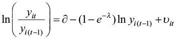
(1)
where y represents real per capita income, υit is the error term, and ∂ is the rate of technological growth which is supposed to be identical for all provinces. The coefficient of initial per capita income (1 – e–λ) decreases for a certain λ since the growth rate declines as per capita income rises. The speed of convergence (λ) determines how quickly Turkish provinces converge towards the steady state. We can re-write the equation (1) by the substitution below[1]:
β = –(1 – e–λ)
(2)
After the replacement (2) into the equation (1), we obtain:
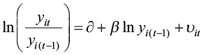
(3)
Then, the following models specify the absolute and conditional models in terms of income, respectively:
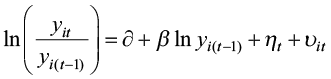
(4)
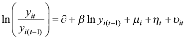
(5)
where μi and ηt stand for unit and time-fixed effects. In other words, the absolute convergence model is interpreted as models that only include time effects, but the conditional convergence model has both unit and time effects (Caselli, 1996; Canova and Marcet, 1995; Rodriguez, 2008). The equation allows us to consider unobservable and unmeasurable components of regional disparities, such as technology. It is not possible to confirm absolute or conditional convergence unless a negative and statistically significant β coefficient is estimated. The existence of convergence implies that poor provinces are likely to grow faster than the rich by converging to a common level of real per capita income. We adapt equations (4) and (5) for public expenditures and tax revenues, respectively, after replacing the dependent variable y with g and t. Fiscal variables should have the same spatial effects on income convergence that are often discovered in earlier research.
As explained before, the parameter λ defined in equations (1) and (2) is the speed or annual rate of convergence. An alternative measure of the convergence process, namely the half-life period (τ), can also be used. It measures the time required for economies to close half of the gap between their steady states (Arbia et al., 2005). The speed of convergence λ is derived from equation (5) as follows which β is estimated from equation (3):
λ = –ln(1 + β)
(6)
Accordingly, the speed of convergence can be considered as follows for the length of the interval is T:
(7)
The measure of the half-life (τ) can be calculated by using the formula below:

(8)
3.2. Spatial models
Anselin (2001) has suggested that it is possible to add the spatial dependence to the basic equations (4) and (5) as an additional regressor, either as a spatially lagged dependent variable or as an error term. Accordingly, it is possible to formulate the main models with the following parameters for explanatory variables and different types of spatial interaction: β (exogenous explanatory variables), ρ (endogenous interaction effect or spatial autoregressive), θ (exogenous interaction effects), and λ (spatial correlation effect of errors or spatial autocorrelation).
The spatial lag models include a spatial lag operator entailing a weighted average of the growth rates in adjacent provinces. It is the product of a spatial weights matrix (W) with the vector of observations of dependent variable y and defined as (Anselin, 2001):
(9)
where wi,j is an element of a fixed and positive N × N spatial weights matrix W. The matrix gives weights that degree the strength of the relationship among pair of spatial units and it is one of the major parts for modelling spatial interdependence between provinces (Le Gallo et al., 2003). The extensive literature on the specification of weights matrices mentions several approaches. It is delicate issue since spatial effects are more robust to the selection of weights matrix than spatial parameters. There are various discussions, however, showing the difficulty of matrix selection, which is subject to technical arguments (Stakhovych and Bijmolt, 2009). Accordingly, the extensive literature on the specification of weights matrices mentions three basic approaches: (i) taking them as completely exogenous structures, (ii) allowing the data to define them, and (iii) estimating them. We follow the first approach which includes examples of spatial contiguity, inverse distance, common border, or centroids. More precisely, we establish a row-standardised simple binary contiguity matrix based on the shared boundary principle. It contains non-zero elements (wij = 1) if provinces have a common border or zero elements (wij = 0) otherwise. The economic reason for this preference is the nature of public expenditures in Türkiye. The expenditures presumably have positive or negative diffusion effects that spread beyond a province’s borders by influencing the well-being of those living in neighbouring provinces. If expenditures have a complementary (for instance, infrastructure and road construction) or substitution (building dams establishing universities, etc.) nature, contiguity becomes more important than distance-based neighbourhood.
Having incorporated spatial weights matrix as a spatial lag operator and spatial correlation terms into the basic model (5), we can define the general static spatial model as follows:
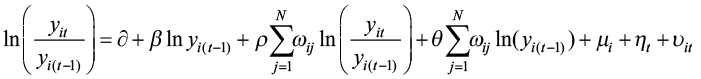
(10)
where 
Based on the constraints of spatial interaction (θ = 0, λ = 0 or ρ = 0), we can derive three forms of spatial lag models. If we assume that endogenous interaction doesn’t exist and spatial externalities matter (ρ = 0), the model becomes the Spatial Durbin Error Model (SDEM). The model is referred to as the Spatial Autocorrelation Model (SAC), if we assume that the parameter for exogenous interaction effects is zero (θ = 0). The parameter θ refers to the spatial lag coefficient of the initial level of income. In this form of the model, however, the β estimators are biased and do not converge when the model includes exogenous interactions of the weights matrix, which signifies the omitted variable bias (Lesage et al., 2009). Moreover, using the same spatial weights matrix for the model might cause weak identification concerns as suggested by Le Gallo (2002). The last form of the model is the Spatial Durbin Model (SDM) when we assume λ = 0. Despite the presence of spatially auto-correlated errors, we have unbiased estimators and valid test statistics in this scenario. Therefore, the model will be more robust against a poor model selection. There are also different sub-models of the SAC and SDM. If we add, for instance, the assumption of λ = 0 to the SAC model, we obtain the Spatial Lag Model (SAR). We can also derive the Spatial Error Model (SEM) by establishing the common factor hypothesis (θ = –ρβ) in the SDM model.
We also employ spatial dynamic models in our analysis of convergence, which include the lag-dependent variable as an explanatory variable in the equation (10). Therefore, the dynamic model in general form is written by extending the model (10) with the lag-dependent variable as follows:
(11)
where
Please note that the model (11) becomes a general spatial static model again when the coefficient of the lag-dependent variable is zero (ψ = 0). Given the dynamic nature of the model, it reveals both short- and long-term effects. Therefore, the estimation results will be reported by their direct (own-province) and indirect (other-province or spill-over) effects. We can attain the Dynamic Spatial Autoregressive Model (DSAR) and the Dynamic Spatial Durbin Model (DSDM), respectively, after imposing the constraints in the cases of the SDM and SAR models to Model (11).
We initially estimate the absolute and conditional convergence models by using the ordinary least squares (OLS) method. The OLS estimation of spatial lag models, however, produces inconsistencies in regression parameter estimates due to the spatially lagged dependent variable, which is always associated with the error term. Therefore, we ought to use the maximum likelihood (ML) method for estimating the spatial lag model (Le Gallo et al., 2003; LeSage and Pace, 2009). Depending on the constraints applied to the equations (11), we use in our analysis both static (the SAR, SEM, and SDM models) and dynamic models (the DSAR and DSDM models). For the most appropriate model selection, we follow the general-to-specific methodology suggested by LeSage and Pace (2009) and Elhorst (2010) and start with the DSDM model as the general specification before applying multiple tests (Lagrange multiplier-LM and likelihood ratio-LR). According to the methodology, we commence using the LM tests. The robust LMρ test from the residuals of the OLS model is used to conclude if there is an autoregressive term (i.e., ρ ≠ 0 and λ = 0). The robust LMλ test is also applied to detect residual autocorrelation (i.e., ρ = 0 and λ ≠ 0). If the LM test results reveal that the use of spatial models is necessary, then we consider the LR test for the most appropriate spatial model selection. Reference can also be made to other tests during model selection. For instance, we test the dynamic spatial model checking whether the coefficient (ψ) of the lag-dependent variable is zero. In addition, information criteria such as the Akaike (AIC) or the Bayesian (BIC) allow us to compare the models that show the most proper fit to the sample data.
3.3. Spatial autocorrelation
The most distinct characteristic of spatial data from others is that they are usually spatially autocorrelated. Spatial autocorrelation is the association between a variable of interest and itself when measured at various places. In this context, Moran’s I is one of the most often used tests for detecting spatial autocorrelation (Moran, 1950). Moran’s I statistic is computed using the formula below and tested against the null hypothesis of no-spatial autocorrelation (i.e., Moran I = 0):
(12)
where I is the Moran I statistic, yi and yj represents variable measure at locations i and j, y̅ is the mean of the variable, S0 indicates the variance ( ) and wij is the spatial weights matrix indexing location of i and j. Please note that N = S0 for a row-standardised weights matrix, as in our study. Moran’s I is a correlation coefficient that indicates the level of spatial autocorrelation in specific data properties. The test is based on geographical covariance, which is then standardized by data variance. It is calculated using a neighbourhood list obtained from a spatial weights matrix. Moran’s I values vary from -1 to 1, where -1 and 1 represent perfect negative or positive spatial autocorrelation, respectively, while 0 shows a random pattern.
4. DATA
The sample comprises 81 provinces in Türkiye from 2004 to 2022. The study uses provincial data in real terms for income, tax revenues, and public expenditures. Turkish Statistical Institute (TurkStat) provides the per capita income statistics from the “National Accounts” database in dollars and the province population data from the “Address Based Population Registration System (ADNKS)”. The Ministry of Treasury and Finance releases data on tax revenues and government expenditures in Turkish lira. After converting all nominal values from local currency to dollars, we use the US consumer price index (2010=100) from the World Bank database to convert all nominal values to real terms. Real values are divided by each province’s population to get the real per capita figures.
The national fiscal policy is characterised by the patterns in tax revenues and government expenditures during the sample period (Fig. 1). First, compared to government expenditures, tax revenues have a steadier income percentage. As an illustration, on the one hand, the tax revenues show an income rate variation of 2.6 percentage points, from 15.4% to 17.9%. Government spending, on the other, varies over time by a larger range (i.e., 6.9 percentage points) between 19.5% and 26.5% of income. Second, the proportions of revenues from taxes and public spending depended on income levels influenced by global macroeconomic trends in the relevant period. For example, from 2008 to 2011, tax revenues fell due to the rapid reduction in income after the global financial crisis. Even though, the percentage of tax revenues to income remained nearly constant. In contrast, the fact that the level of government spending did not decrease compared to previous years caused the share of these expenditures in income to increase. We see a similar progress in the 2019−2021 period.
The third important facet of fiscal policy is shown in Fig. 2. It shows that as average real per capita income falls by province, tax revenues decrease and public spending rises. This means that a smaller portion of public spending is covered by tax revenues; as a result, the government uses more budgetary resources, as well as taxes received from high-income provinces, to support government expenditures in low-income provinces. The government is possibly trying to bridge the development gap across the provinces by putting this policy into effect (Sağbaş, 2002). In conclusion, public spending can be planned centrally and independently of income, in contrast to tax revenues, given Türkiye’s administrative structure and the political preferences of the government.
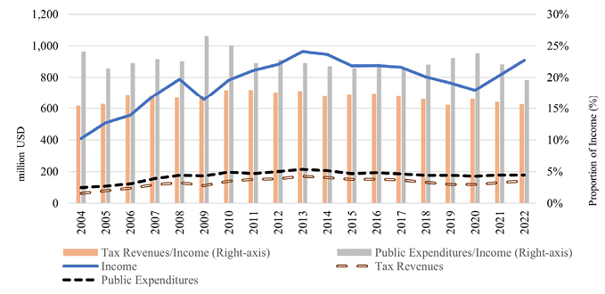
Source: own work based on the data from Turkish Ministry of Treasury and Finance.
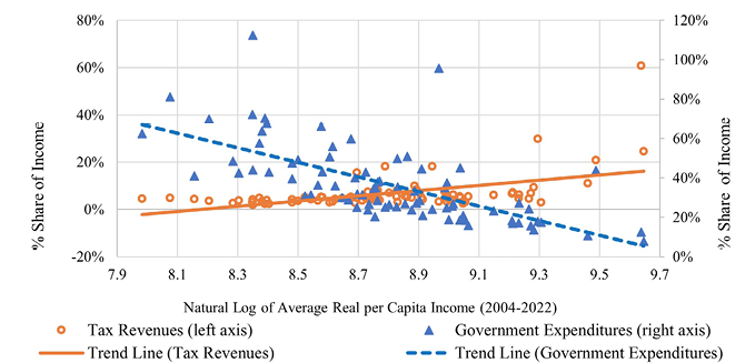
Source: own work based on the data from Turkish Ministry of Treasury and Finance and TurkStat.
Fiscal policies entailing equal distribution of public expenditures and tax burden across a country are important for long-term development. For the tax burden to be shared between regions, public spending should be financed rationally across a country. According to the Statistical Regional Units Classification (NUTS) used for Türkiye, IIBS-1 and IBBS-2 are divided into 12 and 26 subregions, respectively, whereas IBBS-3 (an administrative classification) contains 81 provinces. The 81 provinces chosen for this study allow for a more precise determination of geographic connection among the smaller divisions. As a result, the sample of 81 provinces will be better suited for spatial models, while also providing the ability to work with extensive data compared to other classifications.
We create a balanced and short (time series) panel data set by calculating the natural logarithms of all pertinent values. Reasonably, each lag value used in the models results in the loss of one observation in the sample. As a result, 1,458 observations across 81 provinces for 18 years are there in the statistical analysis. The summary statistics are presented in Table 1. The coefficient of variation expressing the dispersion as a percentage of the mean briefly demonstrates that, out of all the variables, tax revenues in terms of levels and income in terms of growth values have the biggest variation.
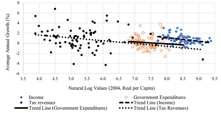
The initial assessment of the validity of our hypotheses is provided by the levels of the variables at the beginning of the year (i.e., 2004) and their yearly average growth rates during the sampling period. Three different kinds of illustrations are prepared for this purpose. The first is placed on the left side of Figures 3, 4, and 5, display the fiscal variables and income distribution for the beginning year. The provincial distribution of their average growth rates throughout the same period is shown in the second illustration, displayed on the right side of Figures 3, 4, and 5. The relationship between annual average growth rates and the natural logarithm of beginning year values is depicted in the third illustration, the dispersion diagram (Fig. 6). In the first two illustrations, the variables get higher values as the shade of red gets darker.
| Variables | Observation | Mean | Std. Error | Min | Max | Coefficient of Variation |
|---|---|---|---|---|---|---|
| ln(yi,t ⁄ yi,t–1) | 1,458 | 0.010 | 0.108 | -0.398 | 0.398 | 14.387 |
| ln(gi,t ⁄ gi,t–1) | 1,458 | 0.001 | 0.109 | -0.583 | 0.739 | 108.700 |
| ln(ti,t ⁄ ti,t–1) | 1,458 | 0.008 | 0.194 | -1.657 | 1.535 | 23.386 |
| ln yi(t–1) | 1,458 | 8.808 | 0.389 | 7.719 | 9.881 | 0.044 |
| ln gi(t–1) | 1,458 | 7.683 | 0.378 | 6.805 | 9.352 | 0.049 |
| ln ti(t–1) | 1,458 | 5.855 | 0.886 | 2.325 | 9.498 | 0.151 |
Source: own work from Stata.
-Enhanced-600dpi.png)
-Enhanced-600dpi.png)
Source: own work based on the data from Turkish Ministry of Treasury and Finance and TurkStat.
-Enhanced-600dpi.png)
-Enhanced-600dpi.png)
Source: own work based on the data from Turkish Ministry of Treasury and Finance and TurkStat.
-Enhanced-600dpi.png)
-Enhanced-600dpi.png)
Source: own work based on the data from Turkish Ministry of Treasury and Finance and TurkStat.
Source: own work based on the data received from the Ministry of Treasury and Finance and TurkStat.
The intense regions in the figures depicting the distribution of income and fiscal variables indicate spatial heterogeneity. The western provinces have higher per capita incomes while the eastern regions have lower ones. Neighbouring provinces have similar income levels, indicating a spatial autocorrelation. These spatial characteristics resemble those of tax revenues. The concentration of public expenditures is shifting towards the eastern provinces. In contrast, the maps showing the average growth rates of the variables reveal that there is weaker spatial interaction between provinces. However, the variables have no polarization across the country.
The real per capita income and tax revenues increased by 0.7% and 0.8% annually on average throughout the sampling period, while the real per capita public expenditures decreased by 0.4%. Figures 3, 4, and 5 show that most provinces with low initial values for all three variables are associated with higher average growth rates. The dispersion diagram (Fig. 6) supports this conclusion. It shows that the starting year values for each of the three variables and the annual average growth rates have a negative connection. Contrary to government expenditures, there is a greater negative correlation between tax revenues and real per capita income.
To assess the spatial correlation of the variables, we additionally compute the Global Moran’s I values (Table 2). At the 1% level, all level variable values are positive and statistically significant. In contrast to fiscal variables, per capita income has a larger value of spatial correlation coefficient. Throughout the relevant period, the coefficient values for per capita public expenditures increased while those for per capita income and tax revenues decreased. However, as the Moran I values are not statistically significant each year, there is no spatial autocorrelation in the growth values of the dependent variables. These outcomes align with the research conducted by Çelebioğlu and Dall’erba (2010) and Gezici and Hewings (2007). Unlike the level values, the growth rates exhibit a relatively weak spatial dependence. The Moran test results are consistent with Figures 3, 4, and 5. As already explained above, a spatial interaction is visible in the maps on the left of the figures showing the levels of the variables on a provincial basis. In contrast, there is no clear evidence of spatial interaction in the maps on the right, which corresponds to the growth rates of the variables.
| Year | ln yi(t–1) | ln gi(t–1) | ln ti(t–1) | ln(yi,t ⁄ yi,t–1) | ln(gi,t ⁄ gi,t–1) | ln(ti,t ⁄ ti,t–1) |
|---|---|---|---|---|---|---|
| 2004 | 0.718* | 0.289* | 0.503* | no data | no data | no data |
| 2005 | 0.734* | 0.308* | 0.502* | -0.006 | -0.093 | 0.224* |
| 2006 | 0.724* | 0.292* | 0.497* | 0.128** | 0.172* | -0.024 |
| 2007 | 0.729* | 0.320* | 0.477* | 0.220* | 0.068 | 0.053 |
| 2008 | 0.736* | 0.355* | 0.477* | 0.213* | 0.233* | -0.034 |
| 2009 | 0.736* | 0.362* | 0.449* | 0.283* | 0.008 | 0.016 |
| 2010 | 0.736* | 0.388* | 0.444* | 0.267* | 0.218* | 0.010 |
| 2011 | 0.724* | 0.381* | 0.441* | -0.040 | -0.029 | 0.112** |
| 2012 | 0.705* | 0.388* | 0.396* | 0.040 | 0.168** | -0.013 |
| 2013 | 0.688* | 0.383* | 0.399* | 0.155** | -0.116 | 0.060*** |
| 2014 | 0.725* | 0.360* | 0.429* | 0.180* | -0.094 | -0.025 |
| 2015 | 0.751* | 0.350* | 0.443* | 0.219* | -0.005 | -0.119*** |
| 2016 | 0.753* | 0.345* | 0.429* | 0.148** | 0.225* | -0.015 |
| 2017 | 0.722* | 0.356* | 0.368* | 0.134** | 0.191* | 0.085 |
| 2018 | 0.714* | 0.339* | 0.309* | 0.080 | 0.235* | 0.080 |
| 2019 | 0.691* | 0.381* | 0.295* | 0.253* | 0.167* | 0.019 |
| 2020 | 0.672* | 0.376* | 0.379* | 0.114*** | 0.103 | 0.108*** |
| 2021 | 0.675* | 0.355* | 0.402* | 0.397* | 0.015 | 0.110*** |
| 2022 | 0.692* | 0.333* | 0.392* | 0.291* | 0.065 | 0.083 |
Note: It is statistically significant at the * p < 0.01, ** p < 0.05 and *** p < 0.10
Source: own work from Stata.
5. RESULTS
The descriptive statistics, on the one hand, confirm that spatial effects might influence income and fiscal variables. On the other, we start by estimating non-spatial models (4) and (5) with the OLS method to understand whether an econometric model that considers spatial effects is required.
5.1. Fixed effects models
We use the models (4) and (5) with time and unit fixed effects (FE) following Barro (2012), Acemoğlu and Molina (2021), and Kremer et al. (2021) in estimating absolute and conditional-beta convergence. The two-way FE model enables to control of unobserved heterogeneity across regions while addressing potential omitted variable bias. The model is especially effective when controlling two types of unobserved heterogeneity (i) that varies across units but is constant over time and (ii) that varies over time but is constant across units. As a result, this approach helps estimate more consistent and unbiased coefficients.
Table 3 displays the OLS estimation results with the Moran and multiple tests (Lagrange multiplier-LM, likelihood ratio-LR). They show that the models are statistically significant based on F values at the 1% level. The values remain significant at the corresponding level once the unit effects are incorporated into the model. According to t and R2 values, almost all fixed effects are statistically significant and adequately explain the models. In our two-way panel fixed effect model, the high R2 value is due to the model’s ability to explain a large portion of the variation in the dependent variable by accounting for both individual and time-fixed effects. These fixed effects control for unobserved heterogeneity across individuals and over time, significantly reducing the residual variance. Also, the p-values less than 0.05 of Moran tests show that the null hypothesis of no spatial autocorrelation is rejected.
| Coefficient of variables | Income | Public expenditures | Tax revenues | |||
|---|---|---|---|---|---|---|
| Absolute | Conditional | Absolute | Conditional | Absolute | Conditional | |
| Constant | 0.278* (0.030) |
2.350* (0.163) |
0.117* (0.032) |
1.775* (0.122) |
0.312* (0.030) |
1.704* (0.118) |
| β, ln yi(t – 1) | -0.012* (0.004) |
-0.256* (0.019) |
no data | no data | no data | no data |
| β, ln gi(t – 1) | no data | no data | -0.007 (0.004) |
-0.240* (0.017) |
no data | no data |
| β, ln ti(t – 1) | no data | no data | no data | no data | -0.015* (0.005) |
-0.255* (0.020) |
| Convergence | 1.3% | 29.6% | No convergence |
27.4% | 1.5% | 29.4% |
| Half-life Period | 55.26 | 2.34 | 2.53 | 45.25 | 2.36 | |
| R2 | 0.81 | 0.84 | 0.75 | 0.79 | 0.41 | 0.48 |
| R̅2 | 0.81 | 0.83 | 0.74 | 0.77 | 0.40 | 0.45 |
| Log-likelihood | 2,395 | 2,501 | 2,165 | 2,297 | 707 | 803 |
| AIC | -4,752 | -4,805 | -4,292 | -4,396 | -1,376 | -1,408 |
| BIC | -4,651 | -4,282 | -4,191 | -3,873 | -1,275 | -885 |
| Time-FE | Yes | Yes | Yes | Yes | Yes | Yes |
| Unit-FE | No | Yes | No | Yes | No | Yes |
| F-test, ∑ηt = 0 | 347.74 (0.000) |
329.53 (0.000) |
242.03 (0.000) |
255.45 (0.000) |
56.48 (0.000) |
51.16 (0.000) |
| F-test, ∑μt = 0 | no data | 2.67 (0.000) |
no data | 3.38 (0.000) |
no data | 2.39 (0.000) |
| Moran I | 0.000 | 0.000 | 0.000 | 0.000 | 0.041 | 0.017 |
| LMρ | 0.000 | 0.000 | 0.000 | 0.000 | 0.050 | 0.030 |
| LMρ (robust) | 0.000 | 0.000 | 0.000 | 0.001 | 0.000 | 0.083 |
| LMλ | 0.000 | 0.000 | 0.000 | 0.002 | 0.061 | 0.083 |
| LMλ (robust) | 0.000 | 0.319 | 0.000 | 0.034 | 0.000 | 0.248 |
| LMρλ | 0.000 | 0.000 | 0.000 | 0.000 | 0.000 | 0.049 |
Note: Values in parentheses below coefficient estimates represent robust standard errors or probabilities in F-test. For spatial autocorrelation tests, the p-value is indicated. It is statistically significant at the * p < 0.01, ** p < 0.05 and *** p < 0.10
Source: own work from Stata.
The findings reveal an absolute convergence of 1.3% and 1.5% annual rates across provinces for per capita income and tax revenues. Based on these estimated rates, the provinces would need approximately 110.5 and 90.5 years to reach the same per capita income and tax revenue, respectively. However, there is no indication of absolute convergence in per capita government spending. The results align with a recent study conducted by Yamanoğlu (2022). He estimated a 2% convergence rate for income and taxes between 2006 and 2020 but found no comparable evidence in government expenditures.
The literature supports that panel data estimates produce results more consistent with conditional-beta convergence, as they consider the individual characteristics of the provinces in the fixed effects component. As a result, we estimate the beta-convergence coefficients for all variables with both unit and time-fixed effects and report the statistically significant results in Table 3. The findings demonstrate that the dependent variables represent conditional convergence on a provincial level and have comparable rates throughout the sample period. As projected, the convergence rates rise to 29.6% for per capita income, 27.4% for per capita public expenditures, and 29.4% for per capita tax revenues. Moreover, provinces would achieve their potential income and tax revenue levels in 4.7 years. For government expenditures, this period is 5.1 years.
Other research using panel data estimations calculates similarly high convergence values. For instance, Yamanoğlu (2022) measured the rate of per capita income at 30%, whereas Filiztekin (1998) and Canova and Marcet (1995) calculated it at 33%. Canova and Marcet (1995) further showed that the convergence coefficient rose to 23% as each region approached its steady state. Similar to this, Tondl (1998) obtained high rates of convergence for the European countries from 1975 to 1996, ranging from 21% to 82%. Elhorst (2010) computed convergence rates of 0.9% and 7.8% for 193 EU regions during the period 1977−2002 by utilising pooled regression and two-way fixed effects models. According to Yamanoğlu (2022), public expenditures and tax revenues have a conditional convergence of 33% and 36% from 2006 to 2020, respectively.
5.2. Spatial models
Following the OLS and ML estimations, we can discuss the result of spatial econometric analysis of beta-convergence for income and fiscal variables separately across Turkish provinces from 2004 to 2022.
We perform the LM tests explained in the methodology section to realize whether there is any spatial error or lag in the models before estimating the spatial models. The robust LM test (LMρ) from the residuals of the OLS model shows an autoregressive term (i.e., ρ ≠ 0) for all models in Table 3. Furthermore, the robust LM test (LMλ) concludes residual autocorrelation (i.e., λ ≠ 0) for the absolute-beta convergence models. We can continue estimating spatial models through the ML methodology since there is either lag or spatial error in all models according to the LM tests. This conclusion is also verified by the (LMρλ) tests.
Table 4 shows the ML results of the five spatial panel models, both dynamic and static, to explain the spatial effects on the convergence of income, government expenditures, and tax revenues. Since a two-way fixed effects model is the appropriate specification, we only focus on their estimation results. The findings from the OLS and ML estimations are consistent. Based on the approach suggested by LeSage and Pace (2009) and Elhorst (2010), the LR tests in Table 5 conclude that the static SEM provides the most appropriate model for all the variables of income, government expenditures, and tax revenues. They have the lowest AIC and BIC scores while the highest log-likelihood values. The absence of divergence in findings between the non-spatial model (OLS) and the SEM suggests that the SEM model specification is precise and does not suffer from an omitted variable problem.
The ML estimation of spatial models suggests that the per capita income growth rate spills over from neighbouring provinces. Therefore, the models measure the total effects that can be divided into two distinct parts: (i) direct effect sourcing from own-province and (ii) indirect effect due to the other provinces or spatial spillover. Nevertheless, these effects are not linked directly with the estimated parameters of spatial models, and hence, they cannot be interpreted as direct or indirect effects. Additional calculations are necessary for gauging these effects. Furthermore, dynamic spatial models permit us to examine both short- and long-run effects (Rios et al., 2017). If only the SEM model is used, however, the usual interpretation of the OLS results is still applicable. Because the SEM model accounts for a general dispersal effect deriving from spatially autocorrelated errors.
| Coefficient of variables | Income | Government expenditures | Tax revenues | ||||||||||||
|---|---|---|---|---|---|---|---|---|---|---|---|---|---|---|---|
| SEM | SAR | SDM | DSAR | DSDM | SEM | SAR | SDM | DSAR | DSDM | SEM | SAR | SDM | DSAR | DSDM | |
| ψ | no data | no data | no data | 0.078* (0.028) |
0.0762* (0.027) |
no data | no data | no data | 0.023 (0.027) |
0.033 (0.027) |
no data | no data | no data | 0.045 (0.029) |
0.051*** (0.029) |
| β | -0.264* (0.018) |
-0.240* (0.018) |
-0.268* (0.019) |
-0.273* (0.020) |
-0.302* (0.021) |
-0.249* (.017) |
-0.238* (0.016) |
-0.260* (0.017) |
-0.250* (0.019) |
-0.272* (0.020) |
-0.258* (0.019) |
-0.254* (0.019) |
-0.262* (0.019) |
-0.277* (0.022) |
-0.288* (0.022) |
| ρ | no data | 0.358* (0.031) |
0.390* (0.031) |
0.359* (0.032) |
0.393* (0.032) |
no data | 0.126* (0.037) |
0.157* (0.037) |
0.133* (0.038) |
0.159* (0.038) |
no data | 0.076*** (0.039) |
0.096* (0.040) |
0.070 (0.038) |
0.093** (0.041) |
| λ | 0.390* (0.033) |
no data | no data | no data | no data | 0.163* (0.037) |
no data | no data | no data | no data | 0.096* (0.040) |
no data | no data | no data | no data |
| θ | no data | no data | 0.141* (0.033) |
no data | 0.148* (0.035) |
no data | no data | 0.110* (0.031) |
no data | 0.098* (0.034) |
no data | no data | 0.081* (0.040) |
no data | 0.094** (0.044) |
| Convergence | 30.7% | 27.4% | 31.1% | 31.8% | 36.0% | 28.6% | 27.1% | 30.1% | 28.7% | 31.7% | 29.8% | 29.3% | 30.5% | 32.45% | 33.93% |
| Half-life period | 2.3 | 2.6 | 2.2 | 2.2 | 1.9 | 2.4 | 2.6 | 2.3 | 2.4 | 2.2 | 2.3 | 2.4 | 2.3 | 2.1 | 2.0 |
| Log-likelihood | 2,568 | 2560 | 2,569 | 2,407 | 2,416 | 2,306 | 2,303 | 2,309 | 2,166 | 2,169 | 806 | 805 | 807 | 735 | 737 |
| AIC | -5,131 | -5,115 | -5,130 | -4,809 | -4,822 | -4,607 | -4,596 | -4,610 | -4,323 | -4,329 | -1,606 | -1,606 | -1,606 | -1,461 | -1,463 |
| BIC | -5,115 | -5,099 | -5,109 | -4,786 | -4,796 | -4,591 | -4,584 | -4,589 | -4,303 | -4,302 | -1,590 | -1,588 | -1,585 | -1,441 | -1,437 |
| Short-run effects | |||||||||||||||
| Direct | no data | no data | no data | -0.283* | -0.300* | no data | no data | no data | -0.252* | -0.271* | no data | no data | no data | -0.279* | -0.287* |
| Indirect | no data | no data | no data | -0.147* | 0.051 | no data | no data | no data | -0.039* | 0.068*** | no data | no data | no data | -0.022*** | 0.079*** |
| Total | no data | no data | no data | -0.430* | -0.249* | no data | no data | no data | -0.291* | -0.203* | no data | no data | no data | -0.301* | -0.209* |
| Long-run effects | |||||||||||||||
| Direct | -0.264* | -0.247* | -0.263* | -0.309* | -0.326* | -0.249* | -0.238* | -0.257* | -0.258* | -0.280* | -0.258* | -0.254* | -0.261* | -0.292* | -0.303* |
| Indirect | no data | -0.126* | 0.053 | -0.181* | 0.041 | no data | -0.033* | 0.077** | -0.041* | 0.068*** | no data | -0.020*** | 0.058 | -0.025*** | 0.082*** |
| Total | no data | -0.372* | -0.211* | -0.490* | -0.284* | no data | -0.271* | -0.180* | -0.299* | -0.212* | no data | -0.274* | -0.203* | -0.316* | -0.221* |
Note: It is statistically significant at the * p < 0.01, ** p < 0.05 and *** p < 0.10. Values in parentheses below coefficient estimates represent robust standard errors or probabilities in F-test and spatial autocorrelation tests
Source: own work from Stata.
| Variables | Test statistics | Null-hypothesis (H0) | Decision | Selected model | |
|---|---|---|---|---|---|
| χ2 | p-value | ||||
| Income | |||||
| SAR vs DSAR | 7,91 | 0.005 | ψ = 0 | Reject | DSAR |
| SDM vs DSDM | 7,71 | 0.006 | ψ = 0 | Reject | DSDM |
| DSAR vs DSDM | 17,76 | 0.000 | θ = 0 | Reject | DSDM |
| SEM vs DSDM | 9,10 | 0.011 | θ = –βλ (θ = –βρ), ψ = 0 | Accept | SEM |
| Government expenditures | |||||
| SAR vs DSAR | 0,73 | 0.394 | ψ = 0 | Accept | SAR |
| SDM vs DSDM | 1,45 | 0.228 | ψ = 0 | Accept | SDM |
| SAR vs SDM | 12,49 | 0.000 | θ = 0 | Reject | SDM |
| SEM vs SDM | 5,46 | 0.020 | θ = –βλ (θ = –βρ), ψ = 0 | Accept | SEM |
| Tax revenues | |||||
| SAR vs DSAR | 2,43 | 0.119 | ψ = 0 | Accept | SAR |
| SDM vs DSDM | 3,16 | 0.075 | ψ = 0 | Accept | SDM |
| SAR vs SDM | 4,09 | 0.043 | θ = 0 | Reject | SDM |
| SEM vs SDM | 2,12 | 0.146 | θ = –βλ (θ = –βρ), ψ = 0 | Reject | SEM |
Note: When performing hypothesis tests, the significance level is set at 0.01. The AIC, BIC and log-likelihood values obtained from the models are also considered to establish the significance level
Source: own work from Stata.
The interpretation of the SEM model is similar to the OLS model but does not provide an estimate of direct effects. Therefore, we might consider an alternative spatial model that can calculate direct and indirect effects. For this reason, we need to evaluate the other spatial models to comprehend the two effects since we consider the SEM model the most appropriate for all variables.
The SEM model infers that the estimated coefficient of the initial per capita income (0.264) from Table 4 is negative and significant, which approves the presence of beta-convergence. This result is consistent with the OLS estimation (0.256) which has already been presented. We utilise the estimated beta coefficient and the direct effect (0.264) to scale the speed of convergence and the half-life for the sampling period. The SEM model provides 30.7% convergence rate and a 2.3 half-life period for per capita income, which are comparable with the OLS results from the non-spatial model (29.6% and 2.3, respectively). This conclusion also proposes that the original model of conditional beta-convergence estimated through the OLS method is not affected by misspecification arising from omitted spatial dependence. According to the positive and significant spatial autocorrelation coefficient (λ = 0.390) from the SEM model, the growth in per capita income in a given province is positively correlated with a shock that occurs in neighboring provinces. Explicitly, there will be a 3.9% change in a given province’s per capita income growth due to a 10% parallel shock in the neighbours.
The estimated β coefficients for the other static and dynamic spatial models in Table 4 are not only negative and statistically significant but also comparable with the SEM model. The lowest (0.240) and highest (0.302) values are obtained from the SAR and DSDM models, respectively. Like the beta-coefficient, the estimated values of spatial externalities (ρ) in Table 4 are significant and positive. The values from different models are consistent, ranging from 0.358 in the SAR model to 0.393 in the DSDM model. The results imply that a 10% change in the rise of per capita income in neighbouring provinces corresponds to an income growth between 3.6% and 3.9% in the relevant province.
The significant and positive θ coefficients for the initial level of income from the SDM (0.141) and DSDM (0.148) models are also very analogous. This interaction appears when a specific province’s effect will depend on the observable peculiarities of its neighbours. The negative and significant direct effects ranging between 0.247 (the SAR model) and 0.326 (the DSDM model) imply the presence of beta-convergence as estimated from the non-spatial model. The direct effect is 0.263 for the SDM and 0.309 for the DSAR models.
The positive and insignificant indirect effects for the SDM (0.053) and the DSDM (0.041) indicate no confirmation of spillover effects. Consequently, the spatial diffusions are presumed to be trivial which suggests that the growth rate of per capita income in a given province is not significantly affected by its neighbours. This conclusion is consistent with the Moran tests found in the descriptive statistics section for the growth rate of per capita income across Türkiye. That said, the SAR and the DSAR models conclude negative and significant indirect effects, which signifies the evidence of dispersion effects. We are cautious about concluding spatial spillover effects due to the mixed results for testing indirect effects. Notwithstanding, the estimated values of total effects for all models are negative and significant. The highest and lowest total effects are estimated for the DSAR and the SDM models (0.490 and 0.211), respectively.
We should also underline that the estimated coefficients of the lag-dependent variable (ψ) for the DSAR and DSDM models are positive and significant. That means the dynamic spatial models might be valid specifications for our analysis. These two models enable us to measure the direct and indirect effects in the short run. The results, however, do not provide any evidence of significant differences between the short-run and long-run.
In conclusion, Table 4 provides comparable results of the estimated spatial coefficients for all models. They are also consistent with the non-spatial model. Therefore, it would be the most effective way to apply information criteria when selecting an alternative spatial model to define the direct and indirect effects. The AIC and the BIC criteria conclude that the SDM model can be considered. The SDM model has not only the lowest AIC (5,130) and the BIC (5,109) scores but also the highest log-likelihood value.
The spatial estimation results from public expenditures and tax revenues agree with the findings obtained from income with a few exceptions. Mind you, the SEM model is chosen as the most appropriate model for all variables according to the LR tests in Table 5. The SEM models confirm beta-convergence for both public expenditures and tax revenues, as is the case of income. Furthermore, these results are consistent with the OLS estimates. The convergence rates and half-life periods are around the values calculated for income. Accordingly, the convergence rates are 28.6% and 29.8% for public expenditures and tax revenues while their half-life scores are 2.4 and 2.3, respectively. The results going along with the OLS verify the absence of an omitted variable bias problem. The positive and significant spatial autocorrelation coefficients (λ) reveal the existence of a positive correlation of the growth in fiscal variables between a given province and its neighbours. However, the strength of this correlation is considerably lower than that of income (3.9%). Indeed, a 10% shock in the neighbouring provinces causes a change of 1.6% in public expenditures and 1.0% in tax revenues in the relevant province.
The negative and statistically significant β and ρ coefficients for the alternative models are not estimated differently from the SEM model. The estimated values of spatial externalities (ρ), however, indicate that a 10% change in the public expenditures of neighbouring provinces leads to an expenditure growth between 1.3% and 1.6% in the relevant province. This impact would be between 0.8%–1.0% for tax revenues.
The θ coefficients for the initial level of income from the SDM and DSDM models are significant and positive. Their values are very similar for the two fiscal variables. The negative and significant direct effects reveal that the presence of conditional beta-convergence is consistent with the non-spatial model. The value of direct effect ranges between 0.238 and 0.280 for public expenditures and -0.254 and -0.303 for tax revenues.
The most important difference in spatial estimates of public expenditures and tax revenues compared to income is to reveal the presence of indirect effects. Therefore, the fact that the growth rates in fiscal variables are affected by neighbouring provinces approves the presence of a spillover effect. However, the estimated values of indirect effects are positive and significant for the SDM and DSDM models while negative and significant for the SAR and DSAR models. In other words, according to the SDM and DSDM models, the impact of neighbouring provinces on the growth of fiscal variables is negative while the SAR and DSAR models indicate that these effects are positive. Accordingly, total effects are reduced by indirect effects in the SDM and DSDM models while being expanded in the SAR and DSAR models. For direct and indirect effects, there are no big differences between the values calculated for the short and long terms.
The difference in spatial estimates for public expenditures and tax revenues stems from dynamic models. The estimated values of the lagged variable in the DSAR and DSDM models for public expenditures are insignificant, unlike income and tax revenues. Therefore, the validity of dynamic spatial models for public expenditures is controversial. Lastly, the AIC and the BIC scores as well as the log-likelihood values indicate that the SDM model can be considered for the interpretation of direct and indirect effects.
We also provide a robustness check to our results through an alternative distance-based neighbourhood matrix. The distance in the matrix is computed between centroids of Turkish provinces. The neighbourhood structures are defined by considering different distances of 250 km, 300 km, 350 km, and 400 km. If the distance is less than 250 km, for instance, it is considered that there is a contiguity relationship between the provinces, and the value is given as 1, otherwise 0. Also, its standardized (normalised) version is used in the analysis. The robust estimation results for the SEM and the SDM models are presented in Table 6.
According to the estimation results obtained from the SEM and the SDM models through the distance-based matrix, the estimated beta coefficients are negative and significant while not varying depending on the distance. Likewise, we find statistically significant results for the spatial coefficients in all models. Moreover, the distance influences the spatial coefficients to a certain extent for all variables. As the number of provinces in the neighbourhood increases, the distance affects the coefficients more. The estimates using the alternative matrix, however, make only the spillover effect (indirect effect) significant differently for public expenditures and tax revenues. The log-likelihood, AIC, and BIC values obtained for the SEM and SDM models are also comparable with the previous estimations.
| Coefficient of variables |
SDM | SEM | ||||||
|---|---|---|---|---|---|---|---|---|
| Distance | Distance | |||||||
| 250 km | 300 km | 350 km | 400 km | 250 km | 300 km | 350 km | 400 km | |
| Income | ||||||||
| β | -0.266* | -0.264* | -0.263* | -0.265* | -0.264* | -0.262* | -0.261* | -0.263* |
| no data | (0.019) | (0.018) | (0.018) | (0.019) | (0.018) | (0.018) | (0.018) | (0.018) |
| ρ | 0.422* | 0.452* | 0.519* | 0.557* | no data | no data | no data | no data |
| no data | (0.034) | (0.038) | (0.041) | (0.043) | no data | no data | no data | no data |
| θ | 0.149* | 0.155* | 0.168* | 0.184* | no data | no data | no data | no data |
| no data | (0.037) | (0.041) | (0.045) | (0.048) | no data | no data | no data | no data |
| λ | no data | no data | no data | no data | 0.423* | 0.452* | 0.519* | 0.558* |
| no data | no data | no data | no data | no data | (0.034) | (0.038) | (0.041) | (0.043) |
| Long-run effects | ||||||||
| Direct | -0.263* | -0.261* | -0.260* | -0.263* | no data | no data | no data | no data |
| Indirect | 0.057 | 0.058 | 0.058 | 0.074 | no data | no data | no data | no data |
| Total | -0.205* | -0.202* | -0.202* | -0.189* | no data | no data | no data | no data |
| Log-likelihood | 2,567 | 2,562 | 2,567 | 2,566 | 2,566 | 2,562 | 2,567 | 2,566 |
| AIC | -5,125 | -5,116 | -5,126 | -5,124 | -5,126 | -5,117 | -5,127 | -5,126 |
| BIC | -5,104 | -5,095 | -5,104 | -5,103 | -5,110 | -5,102 | -5,111 | -5,110 |
| Government expenditures | ||||||||
| β | -0.264* | -0.271* | -0.284* | -0.284* | -0.250* | -0.256* | -0.260* | -0.258* |
| no data | (0.017) | (0.017) | (0.018) | (0.018) | (0.017) | (0.017) | (0.017) | (0.017) |
| ρ | 0.157* | 0.240* | 0.226* | 0.198* | no data | no data | no data | no data |
| no data | (0.042) | (0.048) | (0.054) | (0.061) | no data | no data | no data | no data |
| θ | 0.137* | 0.183* | 0.237* | 0.251* | no data | no data | no data | no data |
| no data | (0.033) | (0.036) | (0.038) | (0.041) | no data | no data | no data | no data |
| λ | no data | no data | no data | no data | 0.169* | 0.260* | 0.270* | 0.257* |
| no data | no data | no data | no data | no data | (0.042) | (0.048) | (0.054) | (0.060) |
| Long-run effects | ||||||||
| Direct | -0.261* | -0.267* | -0.280* | -0.280* | no data | no data | no data | no data |
| Indirect | 0.109 | 0.149* | 0.2163* | 0.238* | no data | no data | no data | no data |
| Total | -0.152* | -0.118* | -0.0631 | -0.042 | no data | no data | no data | no data |
| Log-likelihood | 2,309 | 2,317 | 2,320 | 2,318 | 2,305 | 2,311 | 2,309 | 2,305 |
| AIC | -4,610 | -4,625 | -4,632 | -4,627 | -4,603 | -4,616 | -4,611 | -4,605 |
| BIC | -4,589 | -4,604 | -4,610 | -4,606 | -4,587 | -4,600 | -4,596 | -4,589 |
| Tax revenues | ||||||||
| β | -0.260* | -0.264* | -0.268* | -0.268* | -0.257* | -0.257* | -0.257* | -0.257* |
| no data | (0.019) | (0.019) | (0.019) | (0.020) | (0.019) | (0.019) | (0.019) | (0.019) |
| ρ | 0.115* | 0.129* | 0.162* | 0.180* | no data | no data | no data | no data |
| no data | (0.045) | (0.052) | (0.058) | (0.065) | no data | no data | no data | no data |
| θ | 0.074* | 0.128* | 0.160* | 0.157* | no data | no data | no data | no data |
| no data | (0.042) | (0.047) | (0.049) | (0.052) | no data | no data | no data | no data |
| λ | no data | no data | no data | no data | 0.117* | 0.117* | 0.117* | 0.117* |
| no data | no data | no data | no data | no data | (0.045) | (0.045) | (0.045) | (0.045) |
| Long-run effects | ||||||||
| Direct | -0.258* | -0.262* | -0.266* | -0.266* | no data | no data | no data | no data |
| Indirect | 0.046 | 0.103** | 0.055** | 0.128** | no data | no data | no data | no data |
| Total | -0.212* | -0.159* | -0.055** | -0.138** | no data | no data | no data | no data |
| Log-likelihood | 807 | 808 | 810 | 810 | 806 | 806 | 806 | 806 |
| AIC | -1,606 | -1,609 | -1,613 | -1,611 | -1,607 | -1,607 | -1,607 | -1,607 |
| BIC | -1,585 | -1,588 | -1,591 | -1,590 | -1,591 | -1,591 | -1,591 | -1,591 |
Note: It is statistically significant at the *p < 0.01, **p < 0.05 and ***p < 0.10. Values in parentheses below coefficient estimates represent robust standard errors
Source: own work from Stata.
6. CONCLUSIONS
The study of fiscal convergence on a regional basis is a new topic that extends neoclassical growth models. According to the model, under the balanced budget assumption, government expenditures are funded only by tax revenues, which are a constant fraction of income. As a result, the growth in tax revenues and public expenditures should coincide with income. Although this claim has been validated by several studies, very few studies have employed spatial econometric analysis. Moreover, Solow’s proposition on fiscal policy has been mostly tested across countries or states in federally governed countries. In other words, findings regarding fiscal convergence have been limited to domestic regions or countries where fiscal autonomy is more prevalent.
The use of dynamic panel models is one of the most noteworthy characteristics that distinguishes this study from prior research. Another notable aspect is that the study is carried out for Türkiye, a country with a central government. For this purpose, we use both spatial (static and dynamic) and non-spatial models to investigate the convergence and spatial interactions in income and fiscal variables across Turkish provinces.
The estimation results obtained from the non-spatial fixed effects model partially justify Solow’s proposition. Because absolute convergence could not be determined for per capita public expenditures, unlike per capita income and tax revenues. Earlier studies have yielded mixed results. Our findings are, on the one hand, consistent with, for example, Yamanoğlu (2022). On the other, Saruç et al. (2007) has found strong absolute convergence for public expenditures in their study for the 1990−2005 period but could detect it for tax revenues. Karaş and Karaş (2023) showed an absolute convergence for the fiscal policy by using the variable of tax revenues as a percentage of public expenditures from 2004 to 2020. The convergence rates for per capita income and tax revenues (1.3% and 1.5%, respectively) are calculated in line with previous studies. Yamanoğlu (2022) gaged these rates as 2.0% and 2.1%.
The reason why there is no convergence in public expenditures is presumably that public expenditures do not move together with income. Because the preferences or political inclinations of decision-making institutions or governments, whether centralized or not, can affect national fiscal policies. This outcome differs from the findings obtained from convergence studies conducted across countries or states. Using cross-sectional regression analysis, Scully (1991), Annala (2003), and Coughlin et al. (2007) showed the presence of absolute convergence for income and fiscal variables across states. In contrast, only Couglin et al. (2007) additionally consider spatial dependence in their study. Overall, research on fiscal convergence across states supports the Solow model. Similar results have been identified in studies examining convergence across the EU or OECD countries (Sanz and Velazquez, 2001; Gemmell and Kneller, 2003; Skidmore et al., 2004; Rivero, 2006; Perovic et al., 2016). Among the studies, only Perovic et al. (2016) considered spatial effects and emphasised their importance on fiscal convergence. In studies addressing a larger group of countries, Acemoğlu and Moline (2021) and Kremer et al. (2021) reached results that supported fiscal convergence using non-spatial models.
In the case of Türkiye, tax revenues are expressed as a more fixed or steady fraction of income than government expenditures. The main reason is the fiscal policy instrument of public spending, which the central government has employed to close development gaps among provinces by spending more than the revenues collected. Put another way, taxes collected from high-income regions are transferred to low-income regions. Additionally, budgetary resources other than tax revenues finance government spending. However, there is no fiscal policy that would prohibit tax revenues from remaining a consistent and stable proportion of income. As a result, the absolute convergence estimates for tax revenues in Türkiye yield findings consistent with the Solow model. In contrast, the fact that government expenditures represent changing proportions of income over time violates the Solow model’s assumption, and hence, absolute convergence is not discovered in public spending.
The OLS estimation results of the non-spatial models with time and unit fixed effects validate the conditional convergence. They show that the provinces are approaching their equilibrium rather than a common steady state. The non-spatial model results show that the convergence rates for per capita income, public expenditures, and tax revenues across provinces are 29.6%, 27.4%, and 29.4%, respectively. These rates broadly agree with the findings of the other research that are particular to Türkiye. After following a similar methodology, Yamanoğlu (2022) calculated the convergence rates for the 2006−2020 period as 31.5%, 32.5%, and 36.0%, respectively. The relatively lower calculation of convergence rates in this study is probably due to the longer period examined.
The study addresses whether income, tax revenues, and government spending interact spatially. We use the ML estimation results of the dynamic and static spatial panel models to explain their spatial interactions. The findings from ML estimations are consistent with the OLS results. The comparable results indicate that the models do not suffer from misspecification caused by omitted variable problems. We refer to the SEM and SDM models for the interpretation of the estimation results. According to the most appropriate SEM specification, the convergence rates are computed as 30.7%, 28.6%, and 29.8% for per capita income, public expenditures, and tax revenues, respectively. The negative and significant direct effects expose the existence of conditional beta-convergence which corresponds to the non-spatial model. Because of the inconsistent results for investigating indirect effects, we are hesitant to conclude that spatial spillover effects exist in the short and long terms. However, the total effects for all models are negative and significant. The robustness checks to these results using an alternative distance-based neighbourhood matrix is also provided. The only study suitable for comparison in this field is conducted by Yamanoğlu (2022). He could not find any spatial dependence in per capita tax revenues, unlike per capita income and public expenditures. This result is also probably due to the length of our study period.
Autorzy
REFERENCES
ACEMOĞLU, D. and MOLINA, C. A. (2021), Converging to convergence? A comment, NBER working paper no. 28992. https://doi.org/10.3386/w28992
AKÇAGÜN, P. (2017), ‘Provincial growth in Turkey: A spatial econometric analysis’, Applied Spatial Analysis and Policy, 10, pp. 271–299. https://doi.org/10.1007/s12061-016-9183-5
ALATAŞ, S. and SARI, E. (2021), ‘An empirical investigation on regional disparities in public expenditures: Province level evidence from Turkey’, Social Indicators Research, 158 (1), pp. 217−240. https://doi.org/10.1007/s11205-021-02691-x
ANNALA, C. N. (2003), ‘Have state and local fiscal policies become more alike? Evidence of beta convergence among fiscal policy variables’, Public Finance Review, 31 (2), pp. 144−165. https://doi.org/10.1177/1091142102250327
ANSELIN, L. (2001), ‘Spatial effects in econometric practice in environmental and resource economics’, American Journal of Agricultural Economics, 83 (3), pp. 705−710. http://www.jstor.org/stable/1245103
ARBIA, G. and PIRAS, G. (2005), Convergence in per-capita GDP across European regions using panel data models extended to spatial autocorrelation effects, ISAE working paper no. 51. https://doi.org/10.2139/ssrn.936327
ARBIA, G., BASILE, R. and PIRAS, G. (2005), Using spatial panel data in modelling regional growth and convergence, ISAE working paper no. 55. https://doi.org/10.2139/ssrn.936321
ARBIA, G., LE GALLO, J. and PIRAS, G. (2008), ‘Does evidence on regional economic convergence depend on the estimation strategy? Outcomes from analysis of a set of NUTS2 EU regions’, Spatial Economic Analysis, 3 (2), pp. 209−224. https://doi.org/10.1080/17421770801996664
BARRO, R. J. (2012), Convergence and modernization revisited, NBER working paper no. 18295. https://doi.org/10.3386/w18295
BARRO, R. J. (2016), ‘Economic growth and convergence, applied to China’, China&World Economy, 24 (5), pp. 5−19. https://doi.org/10.1111/cwe.12172
BARRO, R. J. and SALA-I MARTIN, X. (1990), Economic growth and convergence across the United States, NBER working paper no. 3419. https://doi.org/10.3386/w3419
BARRO, R. J. and SALA-I-MARTIN, X. (1992), ‘Convergence’, Journal of Political Economy, 100 (2), pp. 223−251. http://www.jstor.org/stable/2138606
BARRO, R. J. and SALA-I MARTIN, X. (2004), Economic growth second edition, Massachusetts: Cambridge.
BAUMOL, W. J. (1986), ‘Productivity growth, convergence and welfare: What the long run data show’, The American Economic Review, 76 (5), pp. 1072–1085. http://www.jstor.org/stable/1816469
CANOVA, F. and MARCET, A. (1995), The poor stay poor: non-convergence across countries and regions, CEPR discussion paper no. 1265. https://ssrn.com/abstract=289497
CASELLI, F., ESQUIVEL, G. and LEFORT, F. (1996), ‘Reopening the convergence debate: a new look at cross-country growth empirics’, Journal of Economic Growth, 1 (3), pp. 363−389. http://www.jstor.org/stable/40215922
CELEBIOGLU, F. and DALL’ERBA, S. (2010), ‘Spatial disparities across the regions of Turkey: An exploratory spatial data analysis’, Annals of Regional Science, 45 (2), pp. 379–400. https://doi.org/10.1007/s00168-009-0313-8
COUGHLIN, C. C., GARRETT, T. A. and HERNÁNDEZ-MURILLO, R. (2007), ‘Spatial dependence in models of state fiscal policy convergence’, Public Finance Review, 35 (3), pp. 361−384. https://doi.org/10.1177/1091142106295766
DE LA FUENTE, A. (1997), ‘The empirics of growth and convergence: A selective review’, Journal of Economic Dynamics and Control, 21 (1), pp. 23−73. https://doi.org/10.1016/0165-1889(95)00925-6
DE LA FUENTE, A. (2000), Convergence across countries and regions: Theory and empirics, EIB discussion paper no. 2465, http://hdl.handle.net/10419/44793 [accessed on: 21.12.2023].
ELHORST, J. P. (2010), ‘Spatial panel data models’, [in:] FISCHER, M. M. and GETIS, A. (eds), Handbook of applied spatial analysis: Software tools, methods and applications, Berlin: Springer, pp. 377–408. https://doi.org/10.1007/978-3-642-03647-7_19
ELHORST, J. P., PIRAS, G. and ARBIA, G. (2010), ‘Growth and convergence in a multiregional model with space-time dynamics’, Geographical Analysis, 42 (3), pp. 338–355. https://doi.org/10.1111/j.1538-4632.2010.00796.x
ERTUR, C. and KOCH, W. (2007), ‘Technological interdependence and spatial externalities: Theory and evidence’, Journal of Applied Econometrics, 22 (6), pp. 1033−1062. https://doi.org/10.1002/jae.963
EVANS, P. and KIM, J. U. (2014), ‘The spatial dynamics of growth and convergence in Korean regional incomes’, Applied Economics Letters, 21 (16), pp. 1139−1143. https://doi.org/10.1080/13504851.2014.914133
FILIZTEKIN, A. (1998), ‘Convergence across industries and provinces in Turkey’, Ekonomi-Tek, 7 (3), pp. 1−32, https://dergipark.org.tr/en/pub/ekonomitek/issue/61731/922776 [accessed on: 21.12.2023].
GALOR, O. (1996), ‘Convergence? Inferences from theoretical models’, The Economic Journal, 106 (437), pp. 1056−1069. https://www.jstor.org/stable/i339130 [accessed on: 3.12.2023].
GEMMELL, N. and KNELLER, R. (2003), Fiscal policy, growth and convergence in Europe, New Zealand Treasury working paper no. 03/14, https://treasury.govt.nz/sites/default/files/2007-09/twp03-14.pdf [accessed on: 21.10.2023].
GEZICI, F. and HEWINGS, G. J. (2004), ‘Regional convergence and the economic performance of peripheral areas in Turkey’, Review of Urban & Regional Development Studies, 16 (2), pp. 113−132. https://doi.org/10.1111/j.1467-940X.2004.00082.x
GEZICI, F. and HEWINGS, G. J. (2007), ‘Spatial analyses of regional inequalities in Turkey’, European Planning Studies, 15 (3), pp. 383−403. https://doi.org/10.1080/09654310601017091
ISLAM, N. (1995), ‘Growth empirics: A panel data approach’, The Quarterly Journal of Economics, 110 (4), pp. 1127−1170. https://doi.org/10.2307/2946651
KARAŞ, G. and KARAŞ, E. (2023), ‘Testing convergence of fiscal policies in regions of Türkiye’, Ekonomika, 102 (1), pp. 26–40. https://doi.org/10.15388/Ekon.2023.102.1.2
KREMER, M., WILLIS, J. and YOU, Y. (2021), ‘Converging to convergence’, [in:] EICHENBAUM, M. S. and HURST, E. (eds), NBER Macroeconomics Annual 2021, 36, University of Chicago Press, pp. 337−412. https://doi.org/10.1086/718672
LEE, M., LONGMIRE, R., MATYAS, L. and HARRIS, M. (1998), ‘Growth convergence: Some panel data evidence’, Applied Economics, 30 (7), pp. 907−912. https://doi.org/10.1080/000368498325336
LE GALLO, J. (2002), ‘Econométrie spatiale: l’autocorrélation spatiale dans les modèles de régression linéaire’, Economie prévision, 155 (4), pp. 139–157. https://doi.org/10.3406/ecop.2002.6875
LE GALLO, J. and DALL’ERBA, S. (2003), Spatial econometric analysis of the evolution of the European convergence process 1980–1999, working paper no. 0311001, Washington DC: Washington University, https://www.researchgate.net/publication/23749575 [accessed on: 19.12 2023].
LE GALLO, J. and DALL’ERBA, S. (2008), ‘Spatial and sectoral productivity convergence between European Regions, 1975–2000’, Papers in Regional Science, 87 (4), pp. 505−525. https://doi.org/10.1111/j.1435-5957.2007.00159.x
LE GALLO, J., ERTUR, C. and BAUMONT, C. (2003). ‘A Spatial Econometric Analysis of Convergence Across European Regions, 1980–1995’, [in:] FINGLETON, B. (ed.), European Regional Growth, Berlin: Heidelberg, pp. 99−129. https://doi.org/10.1007/978-3-662-07136-6_4
LESAGE, J. and PACE, R. K. (2009), Introduction to spatial econometrics, Chapman and Hall/CRC. https://doi.org/10.4000/rei.3887
MANKIW, N. G., ROMER, D. and WEIL, D. N. (1992), ‘A contribution to the empirics of economic growth’, The Quarterly Journal of Economics, 107 (2), pp. 407−437. https://doi.org/10.2307/2118477
MAZA, A. and VILLAVERDE, J. (2009), ‘Spatial effects on provincial convergence and income distribution in Spain: 1985–2003’, Tijdschrift voor Economische en Sociale Geografie, 100 (3), pp. 316–331. https://doi.org/10.1111/j.1467-9663.2009.00519.x
MORAN, P. A. P. (1950), ‘Notes on Continuous Stochastic Phenomena’, Biometrika, 37 (1/2), pp. 17–23. https://doi.org/10.2307/2332142
PALOMINO, J. and RODRIGUEZ, G. (2019), Peru’s regional growth and convergence in 1979–2017: An empirical spatial panel data analysis, PUCP working paper no. 478. Lima, Peru. https://doi.org/10.18800/2079-8474.0478
PEROVIC, L. M., GOLEM, S. and KOSOR, M. M. (2016), ‘Convergence in government spending components in EU15: A spatial econometric perspective’, Amfiteatru Economic, 18 (42), pp. 240−254. http://hdl.handle.net/10419/168999
PESARAN, M. H., LEE, K. and SMITH, R. (1997), ‘Growth and convergence in a multi-country empirical stochastic Solow model’, Journal of Applied Econometrics, 12 (4), pp. 357−392. https://www.jstor.org/stable/2284959
REY, S. J. and MONTOURI, B. D. (1999), ‘US Regional income convergence: A spatial econometric perspective’, Regional Studies, 33 (2), pp. 143−156. https://doi.org/10.1080/00343409950122945
RIOS, V., PASCUAL, P. and CABASES, F. (2017), ‘What drives local government spending in Spain? A dynamic spatial panel approach’, Spatial Economic Analysis, 12 (2−3), pp. 230–250. https://doi.org/10.1080/17421772.2017.1282166
RIVERO, F. J. D. (2006), Are the tax mix and the fiscal pressure converging in the European Union?, working paper no. 11/06, Spain: Instituto de Estudios Fiscales, https://ideas.repec.org/p/hpe/wpaper/y2006i11.html [accessed on: 12.12.2023].
RODRIGUEZ, J. L. (2008), ‘Regional convergence in the European Union: Results from a panel data model’, Economics Bulletin, 18 (2), pp. 1−7. https://ideas.repec.org/a/ebl/ecbull/eb-08r00001.html [accessed on: 5.12.2023].
ROYUELA, V. and GARCIA, G. A. (2015), ‘Economic and social convergence in Colombia’, Regional Studies, 49 (2), pp. 219−239. https://doi.org/10.1080/00343404.2012.762086
SAĞBAŞ, I. (2002), ‘Türkiye’de Kamu Harcamalarının Yakınsama Üzerindeki Etkisi’, Afyon Kocatepe Üniversitesi İ.İ.B.F. Dergisi, 4 (2), pp. 137–148. https://dergipark.org.tr/tr/pub/akuiibfd/issue/1637/20531 [accessed on: 7.12.2023].
SALA-I-MARTIN, X. (1996), ‘The classical approach to convergence analysis’, The Economic Journal, 106 (437), pp. 1019−1036. https://doi.org/10.2307/2235375
SANZ, I. and VELAZQUEZ, F. J. (2001), The evolution and convergence of the government expenditure composition in the OECD Countries: An analysis of the functional distribution, European Economy Group working paper no. 9/2001, Madrid, Spain, https://www.jstor.org/stable/30025813 [accessed on: 12.12.2023].
SARUÇ, N. T., SAĞBAŞ, I. and CIĞERCI, I. (2007), ‘The geographical distribution of public expenditures and tax revenues in the Turkish case: A convergence analysis’ (conference paper), The Third International Conference on Business, Management and Economics 13 to 17 June 2007, Çeşme- İzmir, Türkiye: Yasar University, Turkey.
SCULLY, G. W. (1991), ‘The Convergence of fiscal regimes and the decline of Tiebout effect’, Public Choice, 72, pp. 51−59. https://doi.org/10.1007/BF00135546
SKIDMORE, M., TOYA, H. and MERRIMAN, D. (2004), ‘Convergence in government spending: Theory and cross‐country evidence’, Kyklos, 57 (4), pp. 587−620. https://doi.org/10.1111/j.0023-5962.2004.00270.x
STAKHOVYCH, S. and BIJMOLT, T. H. (2009), ‘Specification of spatial models: A simulation study on weights matrices’, Papers in Regional Science, 88 (2), pp. 389−409. https://doi.org/10.1111/j.1435-5957.2008.00213.x
TANSEL, A. and GÜNGÖR, N. D. (1998), Economic growth and convergence: An application to the provinces of Turkey, 1975–1995, ERC working paper no. 98/9. https://www.researchgate.net/publication/46453461
TONDL, G. (1998), The Changing Pattern of Regional Convergence in Europe, Robert Schuman Centre no. 97/53, Vienna, Austria. https://doi.org/10.2139/ssrn.130688
YAMANOĞLU, K. B. (2022), Spatial analysis of fiscal convergence between cities and regions in Turkey (Doctoral dissertation), Hacettepe University, https://tez.yok.gov.tr/UlusalTezMerkezi [accessed on: 15.12.2023].
YILDIRIM, J. (2005), ‘Regional policy and economic convergence in Turkey: A spatial data analysis’, 18th European Advanced Studies Institute in Regional Science, 1 (10). https://www.academia.edu/3993186 [accessed on: 11.12.2023].
YILDIRIM, J. and ÖCAL, N. (2006), ‘Income inequality and economic convergence in Turkey’, Transition Studies Review, 13, pp. 559–568. https://doi.org/10.1007/s11300-006-0124-x
YILDIRIM, J., ÖCAL, N. and ÖZYILDIRIM, S. (2009), ‘Income inequality and economic convergence in Turkey: A spatial effect analysis’, International Regional Science Review, 32 (2), pp. 221−254. https://doi.org/10.1177/0160017608331250
FOOTNOTES
- 1 When the log-linearisation method around the steady state is applied to the dynamic capital accumulation equation (k̇/k = s.f(k)/k – (x + n + δ)) in the neoclassical model, the β coefficient is obtained as follows: β = –(1 – e–λ). The parameters in the equation represented by the capital share k, rate of technological progress x, the population growth rate n, and the depreciation rate δ.