Volume 31, 2024, Number 1
https://doi.org/10.18778/1231-1952.31.1.06


Abstract. This article focuses on a very narrowly specific segment of this issue, considering the impacts of HSR in the long term, not as transport arteries connecting the most important metropolitan areas but, on the contrary, as an internal factor of development within a metropolitan region. The paper aims to transfer the present operational European HSR commuting connection frequency experience to a generally applicable frequency estimation formula. Through a quantitative approach, the research analyses the total sample of 1,446 train connections from 10 European metropolitan regions. It answers the secondary research question of what the range of accessibility change between the metropolitan core and the intermediate city is after introducing HSR connection inside metropolitan regions in the time of 1 hour of journey. The estimation model formula calculates the optimal number of HSR connections between the metropolitan core and intermediate city in the HSR developing countries. It is derived and verified from the analysed dataset values. The potential operational change scenarios are presented and described based on the example of 34 metropolitan city pairs.
Key words: metropolitan region, intermediate city, accessibility, frequency, travel time, high-speed rail (HSR).
Society demands speed, efficiency, comfort, and sustainability as vital characteristics of daily travel (McBride, 1996; Cwerner et al., 2009). There is even higher pressure on society nowadays to use sustainable means of transport for daily trips to school, work, and leisure activities. New technologies brought new possibilities for travelling both inside the city and for longer distances.
This paper follows the current political discussion about bringing new opportunities for intermediate cities situated on railways and the challenges mentioned in Martí-Henneberg (2015) about planning and promoting intermodality for intermediate cities and their respective hinterlands, as they need to consolidate their positions as nodal points within the HSR network.
The primary research goal of the presented study is to seek a transferable operational experience for countries developing HSR networks based on the currently developed European HSR operational models. That is why the frequency estimation model will be proposed to estimate a potentially optimal HSR operational frequency based on the sample of 10 European metropolitan regions. In total, 34 city pairs of metropolitan cores and intermediate cities meet the criteria for evaluation. The paper focuses on a specific segment of HSR network operation: HSR commuting delimited by 1 hour of the operational distance between the metropolitan core and the operated intermediate city.
The paper is divided into the following two parts. The first part of the paper (Sections 3 and 4) describes the methods used to create the research dataset and presents the dataset itself. The paper also deals with secondary research questions: firstly, how the range of a daily number of train connections changed when comparing the situations before and after the introduction of HSR connections, and secondly, how travel time changed inside metropolitan regions after the introduction of HSR connections. The second part of the paper (Section 5) presents the frequency estimation model itself and describes the variables used. Subsequently, the model is calibrated by the introduced dataset. The synthesis of the model calibration and dataset analysis results reveal different scenarios of HSR introduction. These scenarios are described afterwards.
The novelty of the presented paper lies in the scale of the analysis dealing with the topic of HSR commuting inside metropolitan regions and primarily in introducing the formula estimating the potential frequency of HSR connections between the metropolitan core and intermediate city. The synthesis of the analytic results brings different scenarios for HSR intra-metropolitan region operational models.
The paper has the following logical structure. Section 2 is framed by the previous research on intermediate HSR stations/cities and the benefits and constraints HSR commuting brings. Section 3 specifies the methodology of the dataset creation and describes the analysed metropolitan dataset. Section 4 presents secondary results according to each case of the studied pairs of a metropolitan core and an intermediate city. Section 5 presents the frequency estimation model and discusses the limits to our analyses and interpretation, and Section 6 concludes the whole.
Albalate and Bel (2012) reviewed several reasons for introducing new HSR infrastructure (travel time reduction between metropolises (Straszak, 1977; Givoni, 2006); overcoming congestions (Barbosa, 2018); improved accessibility of underdeveloped and remote regions (Monzón et al., 2013); and modal split change (Bergantino and Madio, 2020). There is more than one formula for deploying and operating HSR, as Campos and de Rus (2009) and Perl and Goetz (2015) emphasised. It depends on several factors, most importantly geographical conditions (terrain and urbanisation) and historical development, which influence the national policies for HSR implementation (Tapiador et al., 2009; Martí-Henneberg, 2013).
High-speed rail (HSR) was originally designed to compete with air travel between metropolises and to gain a part of the modal split back into trains. Operational distances of 400 to 600 km emerged as competitive (Garmendia et al., 2012a; Givoni and Dobruszkes, 2013; Vickerman, 2015). The priority of the first lines was to make the connection as fast as possible due to economic objectives (Vickerman, 1997; Givoni, 2006). Negative aspects such as the “tunnel effect,” which produces economic disproportions between territories occurred, where only metropolises benefited from the new HSR lines (Vickerman et al., 1999; Gutiérrez et al., 2006; López et al., 2008). The stop policy changed at the next HSR expansion, which made the network denser, and the tunnel effect was partly side-lined. Larger and medium-sized cities and regional centres benefited from the next extension of the HSR network (Ureňa et al., 2009; Vickerman, 2015). Small cities usually avoided these benefits, although some exceptions occurred (Ureňa et al., 2012).
The new segment of HSR operation between metropolis-intermediate/small cities was introduced because the competitive ability of HSR was proved on distances of less than 200 km or around 1 hour (30-90 minutes) of travel time as an alternative to private car trips. (Ureňa at al., 2009; Garmendia et al., 2012b; Vickerman, 2015; Moyano, 2016; Moyano and Dobruszkes; 2017; Matas, 2020). This connection brings new travel opportunities with an essential effect on the resident-workplace location and local economy (Chen and Hall, 2012; Mohíno et al., 2017; Moyano et al., 2019). Blum et al. (1997) have brought a complex economic perspective in their overview, which states that the final effect for the labour market can be very heterogeneous in small cities inside metropolitan areas. Vickerman (2015, p. 158) stated: “In general, although larger and medium-sized cities on high-speed rail links have benefited..., and even some smaller ones on national networks..., the performance of smaller intermediate stations has generally been poor.” Firstly, a HSR station does not need to directly lead to economic development and new firm location in the city (Banister and Berechman, 2001; Albalate and Bel, 2012). Secondly, new HSR stations creating additional conditions (e.g., cheaper building site and salary level) can significantly attract a specific segment of activities (Vickerman and Ulied, 2009; Matas et al., 2020). Thirdly, faster connections can lead to labour migration and people commuting to the metropolis every day (Guirao et al., 2017, 2018). The third scenario is the crucial reason for processing this study.
Several studies have been written on metropolitan commuting and economic opportunities resulting from new HSR stations inside the metropolitan areas. These studies usually focus on Spanish metropolises Madrid and Barcelona (Moyano, 2016; Guirao et al., 2017, 2018) but additionally also on London (Garmendia et al., 2012b), Paris (Mohíno et al., 2018), and German intra-regional commuting (Heuermann and Schmieder, 2014). These studies conclude that the travel time reduction and associated costs/ affordable ticket prices condition the commuting trips. However, other factors also influence travel behaviour and need to be considered. Commuting as a specific travel behaviour concept requires a specific operational timetable regarding time intervals when everyday daily activities begin, mainly in the morning. The principle of a “fast train at the right moment” is unsuitable for everyday commuters with the specific daily rhythms of user activities. Commuting benefits are secured by providing the equivalent train supply for the way back. The number of daily connections or frequency, together with travel time change, are the key quantitative factors influencing the general quality of the connection (L’Hostis and Baptiste, 2006; Moyano, 2016).
The authors state that small cities are most influenced by HSR, and station location (central, lateral, outlying/peripheral) matters for the subsequent city development (Mohíno et al., 2018). Distances of 30 to 200 km (1 hour) are ideal for HSR commuting. These routes are most efficiently served by the particular segment of HSR trains, operated mainly as domestic service with higher-stop frequency and lower ticket prices than long-distance trips (Garmendia, 2012b; Moyano, 2016; Guirao, 2018). The success (occupancy rate) of HSR services depends on the willingness of inhabitants to commute in the context of microeconomic scale conditions such as the unemployment rate, salary level, and housing prices, especially in remote regions (Heuermann and Schmieder, 2014; Guirao, 2017, 2018). The successful implementation of HSR services used by commuters was observed in Great Britain in the case of Ebbsfleet and Ashford stations, and mainly in Spain, where HSR commuting has been a much-discussed topic after the economic crisis in 2008.
Estimating the direct and indirect economic benefits of joining the HSR network is challenging. However, this study does not aim to research the economic effects of a new HSR station. The scope of this paper is the analysis of operational schemas and geographical attributes. Its content indicates the European background of transforming the everyday experience in the HSR developing countries and extending the literature on HSR commuting in metropolitan regions.
The definition of travel time by the new high-speed rail service between the metropolitan core and the intermediate city is the key factor for the study. One-hour travel was defined as the default condition to include such an HSR connection in our data sample for analysis. This condition corresponds to the expected typical working day. It can be assumed that usual working hours lie between 8 and 12 hours daily. Working hours are commonly scheduled during the day, so night trains were excluded. Under this assumption, seven services constitute regular high-speed services once per two hours to the station. This minimum service frequency allows reliable daily commuting connections, not only for work activities. High-speed services are often operated on various routes from smaller towns in the morning and back from metropolitan areas in the afternoon to meet specific demands from commuters during specific times. The frequency of seven daily services indicates a stronger relationship between the intermediate regional city and the metropolis, which can also be supplied by two other services - before and after working hours.
As the research focuses on the extent to which time accessibility benefits residents of regional cities in the hinterland of metropolitan cities based on participation in an HSR system, population thresholds were also established for selecting regional centres. A city’s population had to be no more than 50% of a metropolitan city and no larger than 500,000 inhabitants, which corresponds to the usually simplified threshold for the existence of a metropolitan core in a city system in European conditions (Moreno-Monroy et al., 2021). Therefore, cities such as Turin were not included in the research as the benefits of connecting it to Milan by HSR would be less substantial for cities with populations in the tens or hundreds of thousands. Only the travel time for a direct connection of the fastest tier of trains was considered. It can be assumed that when traveling to/from metropolitan cities, people want to spend as little time as possible on the train.
The research data was based on two primary sources. The European Rail Timetable (2019, formerly known as the Thomas Cook European Timetable), which provides timetables for selected rail lines in all European countries, was used as the source for the high-speed analysis. The data spans from October 2019 until recently and is thus not biased by the Covid-19 pandemic. The data for conventional train services was then based on the historical records of the European Rail Timetable, working with the years before the construction of HSR on the studied routes, precisely 1978, 1987, 1995, 2000, 2005, and 2010 (Fig. 1).

Fig. 1. Cities and railways included in the study
Source: European Rail Timetable, 2019; RRG GIS Database, 2022; own work.
The resulting data sample, on which the research is based, contains data on all conventional and high-speed connections for each identified relevant pair of a metropolitan core and an intermediate regional city. The database contains 34 metropolitan core–intermediate city pairs, for which 1,464 connections were recorded (737 conventional and 727 high-speed), including their total travel times. For the conventional connections, 114 connections were excluded from further analysis based on the assumption that the travel times of the connection were too long compared to other available connections. The long travel times for these services were accompanied by stops at many intermediate stations. Therefore, it can be assumed that these services would not be used for transport along the entire route but primarily serve intermediate stops. The following conditions, therefore, applied to conventional services for inclusion in further analyses:

where T is the travel time, n/N is the number of conventional services on the given metropolitan-urban route, and x is the travel time on the nth service.
The change in the accessibility of metropolitan cities through HSR was measured based on two leading indicators: travel times and the frequency offered. These indicators for HSR were compared with the operation of conventional trains before the construction of HSR. As a result, the benefits of HSR in terms of time availability can be described. Travel times on high-speed lines were primarily calculated between HSR stations. When there was more than one HSR station in a metropolitan city, the travel time was calculated for the more centrally located station (e.g., in Milan: Milano Centrale was considered rather than Milano Rogoredo).
Travel times were calculated similarly for conventional connections. Time was calculated between the central station at the origin (an intermediate city) and the central station at the destination (a metropolitan city). Although the authors acknowledge the importance of the “first and last miles” to the total travel time, these were not included in the accessibility analyses for several reasons. The first and last miles are the equivalent of door-to-door transportation (Monzón et al., 2016), typically done by road. However, this mode of transport was not investigated in this research. The second reason is that the research only dealt with rail transport; passengers must travel to a rail station in both cases. The general overview of city pairs with essential characteristics is presented in Table 1.
| Origin metropolis | Destination | HSR opening year | Time-table source | Popu-lation (k.) | Station location | Distance (km) | Frequency | Travel time (min.) | Travel time (max.) | Travel time (avg.) | |||||
|---|---|---|---|---|---|---|---|---|---|---|---|---|---|---|---|
| HSR | C-H | HSR | C-H | HSR | C-H | HSR | C-H | HSR | C-H | ||||||
| Milano | Reggio Emilia | 2008 | 2005 | 161 | P | 151 | 157 | 27 | 20 | 40 | 83 | 53 | 112 | 48 | 99 |
| Bologna | 2008 | 2005 | 371 | C | 215 | 219 | 51 | 32 | 59 | 105 | 77 | 144 | 67 | 117 | |
| Brescia | 2007 | 2005 | 190 | C | 83 | 83 | 33 | 24 | 38 | 50 | 48 | 64 | 39 | 52 | |
| Desenzano del Garda | 2007 | 2005 | 27 | L | 111 | 111 | 16 | 30 | 53 | 68 | 53 | 84 | 53 | 76 | |
| Peschiera del Garda | 2007 | 2005 | 10 | L | 125 | 125 | 17 | 31 | 57 | 70 | 69 | 94 | 60 | 85 | |
| Madrid | Guadalajara-Yebes | 2003 | 2000 | 85 | P | 64 | 54 | 9 | 13 | 23 | 31 | 27 | 42 | 25 | 35 |
| Calatayud | 2003 | 2000 | 21 | L | 221 | 242 | 9 | 7 | 56 | 127 | 76 | 146 | 65 | 135 | |
| Cuenca Fernando Zóbel | 2010 | 2005 | 55 | P | 189 | 201 | 15 | 3 | 52 | 146 | 70 | 161 | 62 | 151 | |
| Ciudad Real | 1992 | 1987 | 74 | L | 171 | 176 | 15 | 4 | 51 | 148 | 62 | 161 | 53 | 152 | |
| Toledo | 2005 | 2000 | 82 | L | 75 | 99 | 15 | 7 | 31 | 60 | 33 | 77 | 33 | 67 | |
| Segovia | 2007 | 2005 | 55 | P | 68 | 108 | 28 | 7 | 27 | 116 | 32 | 129 | 29 | 122 | |
| Valladolid | 2007 | 2005 | 312 | C | 180 | 250 | 31 | 14 | 54 | 144 | 78 | 161 | 64 | 150 | |
| Barcelona | Camp de Taragona | 2008 | 2005 | 131 | P | 95 | 93 | 26 | 39 | 32 | 48 | 42 | 71 | 35 | 56 |
| Lleida | 2008 | 2005 | 135 | C | 174 | 150 | 25 | 13 | 58 | 119 | 82 | 152 | 66 | 137 | |
| Girona | 2013 | 2010 | 94 | C | 95 | 102 | 15 | 22 | 40 | 82 | 41 | 96 | 41 | 88 | |
| Figueres Vilafant | 2013 | 2010 | 46 | L | 129 | 143 | 15 | 13 | 55 | 112 | 58 | 125 | 56 | 114 | |
| Paris | Lille | 1993 | 1987 | 229 | C | 237 | 258 | 21 | 11 | 59 | 119 | 77 | 133 | 62 | 126 |
| Reims | 2007 | 2005 | 179 | C | 147 | 173 | 14* | 8 | 39 | 93 | 46 | 98 | 44 | 95 | |
| Le Mans | 1990 | 1987 | 142 | C | 202 | 211 | 7 | 22 | 63 | 99 | 64 | 138 | 63 | 112 | |
| Vendome | 1990 | 1987 | 17 | P | 162 | - | 12 | - | 45 | - | 52 | - | 50 | - | |
| Lyon | Valence TGV | 1994 | 1987 | 95 | P | 104 | 105 | 17 | 19 | 36 | 50 | 47 | 72 | 40 | 57 |
| Le Creusot | 1983 | 1978 | 23 | P | 129 | - | 7 | - | 42 | - | 50 | - | 45 | - | |
| Avignon | 1994 | 1987 | 90 | L | 234 | 230 | 15 | 15 | 63 | 115 | 82 | 151 | 70 | 125 | |
| Berlin | Wolfsburg | 1998 | 1995 | 121 | C | 183 | ? | 29 | 4 | 63 | 162 | 87 | 162 | 75 | 162 |
| Frankfurt | Limburg | 2002 | 2000 | 34 | C | 70 | 70 | 12 | 13 | 30 | 61 | 37 | 67 | 33 | 67 |
| Montabaur | 2002 | - | 12 | L | 92 | - | 12 | - | 41 | - | 50 | - | 45 | - | |
| Bonn/Siegburg | 2002 | 2000 | 325 | P | 155 | 197 | 14 | 17 | 52 | 113 | 71 | 114 | 62 | 113 | |
| London | Ashford | 2003 | 2000 | 67 | C | 90 | 90 | 46 | 31 | 30 | 65 | 44 | 84 | 39 | 73 |
| Folkestone | 2003 | 2000 | 51 | C | 112 | 113 | 21 | 24 | 53 | 89 | 63 | 101 | 55 | 93 | |
| Dover | 2003 | 2000 | 41 | C | 124 | 124 | 21 | 44 | 64 | 99 | 74 | 119 | 66 | 108 | |
| Canterbury | 2003 | 2000 | 55 | C | 112 | 113 | 20 | 37 | 52 | 83 | 60 | 109 | 57 | 92 | |
| Ramsgate | 2003 | 2000 | 41 | C | 140 | 128 | 20 | 25 | 71 | 104 | 81 | 119 | 76 | 112 | |
| Amsterdam | Breda | 2007 | 2005 | 173 | C | 117 | 132 | 50 | 31 | 67 | 118 | 72 | 121 | 68 | 121 |
| Brussels | Liege | 2002 | 2000 | 194 | L | 105 | 103 | 42 | 19 | 46 | 80 | 65 | 80 | 59 | 80 |
Note: C - central, L - lateral, P - peripheral[1], C-H - conventional-historical
Source: The European Rail Timetable (2019 and 1978, 1987, 1995, 2000, 2005, 2010), European Union, 1995-2023, own work.
In this section, the research results are presented. The individual transport markets linked to each of the selected metropolitan areas are considered individually for each metropolitan area, for which the relationship with the relevant regional terminals is assessed in aggregate. Relevant transport markets are characterised in Table 1.
The first case focuses on the Spanish metropolises of Madrid and Barcelona (cases 1 and 2 in Fig. 2). Regarding Madrid, the introduction of HSR increased the frequency to all selected terminals except Guadalajara, where more conventional connections were operated than high-speed connections. Regarding the total frequency, Madrid saw them more than double (an increase of 122%). The average travel time on HSR was 55% below the average on conventional services, considered the fastest conventional service one quarter (26%) below the original time. In Barcelona, the situation was somewhat different since of the four routes studied, only two, i.e., to Girona and Lleida, saw an increase in connections due to the introduction of HSR. In particular, the number of conventional connections to Camp de Tarragona was initially at a substantial level. As a result, the number of high-speed connections on the routes examined for Barcelona reached only 93% of the original number of conventional connections. However, substantial time savings were recorded, with the average travel time being reduced by 42% of the original travel time and the fastest service by a third (33%) of the original time.

Fig. 2. Metropolitan cases 1 and 2: Madrid and Barcelona – frequency and travel time range – comparison of HSR and conventional trains
Cases 3, 4, and 5 in Fig. 3 present the results for the metropolitan core–intermediate city pairs linked to crucial international high-speed links, namely London, Brussels, and Amsterdam. In the case of London, five routes were considered, of which only one, Ashford, saw an increase in connections due to the introduction of HSR (46 HSR/ 31 conv.). In contrast, the number of HSR connections did not reach the conventional numbers for the others. Overall, the number of HSR services was 80% of the original conventional services. However, average travel times fell by less than half (43%) of the original travel times. One connection was always considered in the case of the other two metropolises shown in Fig. 3. On the Brussels–Liege route, the introduction of HSR more than doubled the frequency (an increase of 121%) and reduced the average travel time by about a quarter (27%). On the Amsterdam–Breda route, HSR increased services by 61% and reduced the average travel time by less than half (44%).

Fig. 3. Metropolitan cases 3, 4, and 5: London, Brussels, and Amsterdam – frequency and travel time range – comparison of HSR and conventional trains
Cases 6 and 7 in Fig. 4 show the results for two French metropolises, Paris and Lyon, which are also connected by a critical long-distance HSR artery linking these two major French metropolises. It is worth mentioning that these French cases have a very long period of impact. These lines were introduced in the previous century (except for Paris–Reims) and cover the oldest HSR connection on the crucial line between Paris and Lyon, here connected to Lyon: Le Creusot, where HSR was introduced in 1981. In the case of Paris, four linkages with HSR services were considered, with the line to Le Mans recording only 32% of the original number of conventional services. The services to Lille and Reims saw substantial increases, and the one to Vendome saw the introduction of entirely new services. Overall, introducing HSR increased services by a third (32%) while halving the average travel time (a reduction of 51%). In the case of Lyon, three services were considered: the line to Avignon, where the introduction of HSR did not change the number of services; the line to Valence, where the number of HSR services was lower than the original conventional services; and the line to Le Creusot, where completely new services were introduced. Overall, the number of services increased by 15%, and the average travel time fell by less than a half (40%). Even the fastest service fell by less than three quarters to 28% of the original conventional time.

Fig. 4. Metropolitan cases 6 and 7: Paris and Lyon – frequency and travel time range – comparison of HSR and conventional trains
The last of the graphs presenting the results for individual sessions (cases 8, 9, and 10 in Fig. 5) shows the results for the metropolitan areas of Milan, Berlin, and Frankfurt. In the case of Milan, five linkages with HSR services were examined, three of which showed a substantial increase in the frequency, namely to Bologna, Brescia, and Reggio Emilia. The lines to Desenzano del Garda and Peschiera del Garda showed fewer HSR connections than conventional ones. However, it should be noted that these two services are essentially tourist destinations used by many Milanese for weekend holidays, for which conventional services appear sufficient, given the short distances involved. The average travel time for Milan-bound services fell by about a third (37%); even the fastest travel time fell by less than a quarter (24%) of the original conventional travel time. In the case of Berlin, one connection to Wolfsburg was considered, where the frequency increased substantially to more than seven times the original (an increase of 625%), and the average travel time fell by about a half (54%). The last metropolitan area examined was Frankfurt am Main, where three services were considered, one of which, to Montabaur, involved the introduction of entirely new services, while the remaining two, to Bonn and Limburg, had slightly fewer high-speed services than conventional services, with an overall increase of 27% in the number of services and a fall in average travel times by less than a half (49%).

Fig. 5. Metropolitan cases 8, 9 and 10: Milano, Berlin, and Frankfurt – frequency and travel time range – comparison of HSR and conventional trains
Source figures 2 to 5: European Rail Timetable, 2019; own work.
In summary (Fig. 6), the frequency increased by 17% due to the construction and introduction of HSR. Another benefit to the routes studied on metropolitan core–intermediate city relationships was the average time savings of 43%. Therefore, these routes do not reflect long-distance traffic but everyday commuter traffic. It should be added that the routes studied range from 64 to 237 km, and the average distance on all routes studied was 137 km. The average reduction of 43% in commuting time to or from a metropolitan core is a relatively substantial benefit. Especially since it is on shorter distances, time savings are more difficult to achieve. However, at these distances, the most massive traffic flows occur. In contrast, long-distance transport may be more subject to seasonal influences and may reflect other characteristics according to the metropolitan areas it connects.


Fig. 6. Summary comparison of HSR and conventional lines
Source: European Rail Timetable (2019); own work.
In the 34 pairs of metropolitan cores with intermediate cities representing 10 metropolitan regions in 7 different countries, which are associated with different institutional approaches to the planning and construction of HSR lines, it can be observed that the benefits varied somewhat according to the examples analysed. Although the overall impact shown in Fig. 6 is substantial, it should be noted that it depends very much on the specific situation of each link analysed. Based on the analysis, these connections can be divided into several categories according to the initial conditions of each pair of a metropolitan core and an intermediate city (see Table 2).
The possible role of the HSR introduction:
A. New connections: This is an essential category where the introduction of HSR through a completely new route brought the possibility of a connection for a new location that did not have a direct rail connection in the past (Frankfurt–Montabaur, Lyon–Le Creusot, Paris–Vendome). This category is based on the exclusive position of HSR connections, for which there is no competition in the form of existing conventional rail links.
B. Marginalisation of the conventional connection offer: This category represents situations where HSR connections substantially increase connection frequency. This way they represent an entirely new role in offering rail connections for which conventional rail is not competitive in terms of either frequency or travel time. Therefore, the conventional part of the rail links was marginalised, and it can be assumed that the main objective of these conventional links was to serve additional intermediate stops of even lesser importance. Examples of such connections include Berlin–Wolfsburg, Madrid–Cuenca, Madrid–Segovia, Madrid–Ciudad Real, Madrid–Valladolid, Brussels–Liege, Madrid–Toledo. There was a considerable increase in service for these pairs, at least roughly double the frequency compared to the original conventional railway.
C. Substantial predominance of HSR connections: In this category, HSR connections substantially increased the serviceability of a given intermediate city. However, it cannot be unequivocally said that this was such a fundamental marginalisation of conventional rail as in the previous case. Nonetheless, it is possible to support the claim that HSR also brought a substantial change in speed and service. Examples of such connections include Barcelona–Lleida, and Paris–Lille. Paris–Reims, Amsterdam–Breda, Milan–Bologna, London–Ashford, Milan–Brescia, and Milan–Reggio Emilia. In this category, there was an increase in services through the introduction of HSR.
D. Balancing the conventional connection supply: This category represents situations where HSR connections took over a substantial part of the transport supply and had an overall share of around half of the number of rail connections. There was also a certain complementarity of supply, but with much more substantial effects on the overall structure of the services offered. Although conventional rail links were probably not equivalent, they were still substitute products, although conventional rail links were probably not equivalent but still a substitute product. Examples of such connections include Madrid–Calatayud, Barcelona–Figueres, Lyon–Avignon, Frankfurt–Limburg, Lyon–Valence, London–Folkestone, Frankfurt–Bonn, and London–Ramsgate. In this category, HSR connections showed service levels between 70% and 100% of the original conventional service.
E. Supplementing the conventional connection supply: This category represents situations where conventional railways offered above-standard connection frequencies, so HSR connections were only a particular supplement to transport services. Their target group was only a selected minority segment. The existing conventional railways continued to be used widely. This situation naturally presupposes the parallel operation of conventional and HSR connections. Examples include the heavily used Madrid–Guadalajara, Barcelona–Girona, Barcelona–Camp de Tarragona, Milan–Peschiera del Garda, London–Canterbury, Milan–Desenzano del Garda, London–Dover, and Paris–Le Mans lines. HSR connections showed service levels at less than 70% of the original conventional service in this category. It is clear from the above list that the Milan connections were widespread destinations used extensively for suburban tourism by the Milanese, while the Barcelona and London connections were essential destinations resulting from work commutes. Nevertheless, even in these cases, HSR brought entirely new quality in substantially reduced travel times.
| type | route | HSR connections | change | type | route | HSR connections | change |
|---|---|---|---|---|---|---|---|
| A | Frankfurt – Montabaur | 12 | - | C | Milano – Reggio Emilia | 47 | 135.00 |
| A | Lyon – Le Creusot | 7 | - | D | Madrid – Calatayud | 16 | 128.57 |
| A | Paris – Vendome | 12 | - | D | Barcelona – Figueres | 28 | 115.38 |
| B | Berlin – Wolfsburg | 33 | 725.00 | D | Lyon – Avignon | 30 | 100.00 |
| B | Madrid – Cuenca | 18 | 500.00 | D | Frankfurt – Limburg | 25 | 92.31 |
| B | Madrid – Segovia | 35 | 400.00 | D | Lyon – Valence | 36 | 89.47 |
| B | Madrid – Ciudad Real | 19 | 375.00 | D | London – Folkestone | 45 | 87.50 |
| B | Madrid – Valladolid | 45 | 221.43 | D | Frankfurt – Bonn | 31 | 82.35 |
| B | Brussels – Liege | 61 | 221.05 | D | London – Ramsgate | 45 | 80.00 |
| B | Madrid – Toledo | 22 | 214.29 | E | Madrid – Guadalajara | 22 | 69.23 |
| B | Barcelona – Lleida | 38 | 192.31 | E | Barcelona – Girona | 37 | 68.18 |
| B | Paris – Lille | 32 | 190.91 | E | Barcelona – Camp de Taragona | 65 | 66.67 |
| C | Paris – Reims | 22 | 175.00 | E | Milano – Peschiera del Garda | 48 | 54.84 |
| C | Amsterdam – Breda | 81 | 161.29 | E | London – Canterbury | 57 | 54.05 |
| C | Milano – Bologna | 83 | 159.38 | E | Milano – Desenzano del Garda | 30 | 53.33 |
| C | London – Ashford | 77 | 148.39 | E | London – Dover | 65 | 47.73 |
| C | Milano – Brescia | 57 | 137.50 | E | Paris – Le Mans | 29 | 31.82 |
Source: The European Rail Timetable (2019 and 1978, 1987, 1995, 2000, 2005, 2010), own work.
The above typology of the identified intra-metropolitan systems of HSR connections cannot, by its nature, cover all institutional, geographical, technical, and socio-economic aspects. Therefore, some of the links analysed are on the edge between two categories, and it could be somewhat problematic to classify them into one of the categories strictly. Examples include Madrid–Calatayud balancing categories C and D with an increase in services of 29%, and the Madrid–Guadalajara line on the border between categories D and E with HSR services at 69% of the original conventional level.
The result of the analysis of the frequency and time changes determined by the introduction of the high-speed connection is an important prerequisite for the planning of possible further construction of high-speed lines in the future, and especially for planning the prioritisation and efficiency of regional high-speed terminals in medium-sized cities. The following frequency estimation model represents the transformation of the results into a potentially applicable planning framework. Thus, the frequency estimation model is proposed to estimate a potentially optimal HSR operational frequency for countries developing HSR networks based on the currently developed European HSR systems. As presented in Section 4, according to several scenarios for the role of HSR inside metropolitan regions mentioned above.
Simple gravity model introduced by Anderson (1979) and applied primarily to identify trade flows is in the beginning of the study. However, the model has been applied to transport issues. Its underlying variation reflects economic or population importance and geographical proximity measured by time or distance. The basic gravity model for transport flows is determined as follows:

where F is the transport flow, G is the constant, POPi is the population of city i, POPj is the population of city j, and Dij is the distance between cities i and j.
The Frequency estimation model comes from the simple gravity model. Frequency is used as a proxy for transport flow, while there is no data available on the number of passengers covering historical milestones from the years when HSR was launched on the routes (starting in 1978 and finishing in 2010). The estimated relation between the metropolitan core and relevant intermediate city as the assumption for the frequency is expressed as ERPn … which is the estimated relation power of city pair on the specific transport market or route[2] in the analysed sample. In the next step, the model was augmented to reflect more variables covering the conditions on the route before the introduction of HSR. As a result, the standard combination of traditional variables was used in the model, coming from the dataset mentioned in section 3 Data and methods.
First, the size of the market expressed as POPt …is a sum of the metropolitan core and the relevant intermediate city population because it reflects the size of such a transport market, and it is raised to the power of two to emphasize the strength of these two cities. The second traditional variable is the distance between the metropolitan core and the intermediate city expressed as D… which is the rail route distance of a given train between the metropolitan core and the relevant intermediate city in kilometres.
Further, the model was augmented with variables reflecting starting conditions and other principal contextual factors on the route as a next step. As the first substantial variable, the travel time of a given rail connection was used and expressed as Tr … which is the travel time by a train on the route between the metropolitan core and the relevant city of a train connection. This travel time enables one to identify the potential benefits achieved by launching high-speed trains on a given transport market or rather a given route for end-users or commuters. As the next step, the direct train’s slowest original conventional travel time was used and expressed as a Tmax… which is the maximum conventional train time before high-speed introduction on the route between the metropolitan cores and the relevant city. This variable enables the authors to assess the range of potential benefits for passengers because the slower the original conventional rail was, the higher the potential benefit of high-speed introduction. The reason for putting this variable to the numerator is that it potentially increases the benefits expressed in our model as frequency, reflecting the reaction of demand of passengers.
From the two variables mentioned above, the variable Tmax-dif was derived, which is the ratio of the travel time of a train (both conventional or high-speed) connection compared to the maximum travel time by conventional train between a metropolitan core and a relevant city. This variable enables one to identify the range of individual benefits of each train connection faster than the slowest one. It means that the faster the train connection, the lower the ratio is, and that is the reason to put this variable to the denominator, because faster trains increase the potential benefit. The last variable reflecting the context and the significance of the change achieved by the introduction of high-speed connection is variable Ttrain-road … which is the ratio of the travel time of a train (both conventional or high-speed) connection compared to the travel time by car between the metropolitan core and a relevant city. It is defined as a ratio of travel time by a train connection divided by the travel time by car. In other words, the slower the original train connections, the greater the potential benefit. Thus, this variable is reflected in the numerator. To achieve the balance of the model in accordance with the substance of used variables in the numerator (meaning Tmax and Ttrain-road) based on travel time, both time-derived variables used in the denominator by two (meaning Tr and Tmax-dif) were raised.
The last variable used in the model reflects the balance of size or power of a metropolitan core and an intermediate city, because the smaller the intermediate city is, the lower the motivation to operate the HSR stop there. It is defined as POPdif … which is the share of the relevant intermediate city population to the metropolitan core population. It means that the smaller the intermediate city is, potentially lower the benefits are. Thus, it decreases the motivation for higher frequency. This variable is consistently put in the numerator because it corrects the market size as the abovementioned total.
Finally, the model according to the logic above reflects the frequency change in the new state compared to the original state with a conventional rail link, while frequency is considered as a proxy for potential benefits from the introduction of the HSR connection.
The formula for the estimated relation power ERPn of the city pair on the specific route is expressed as:

The results of the equation were normalised by range (Min-Max Normalisation) according to the following equation:

Thus, the resulting values of ERPhsrn-normalised … lie in the interval {0,1}. The HSR frequency estimation formula is based on an estimated linear trend capturing the relationship between the actual number of HSR connections and Estimated Relation Power (ERP), see Fig. 7, which can be defined as a standard equation of the line:
y = a * x + b
where coefficient a = 68.493, variable x = ERP, and constant b = 9.048
The frequency estimation model equity:
FE = 68.493 * ERPhsrn-normalised + 9.048
where FE is the frequency estimation of HSR connections on the specific route[3]. The standard deviation in our model achieved 15.07, but it varies from less than two to twenty in different groups. The model was verified using a total sample of 1,464 connections included in the analysed dataset.
The operational HSR frequency of every 34 metropolitan core–intermediate city pairs was compared in Fig. 7 with the estimated frequency gained by the model formula. The presented verified results show the intersperse by the linear regression curve–the model defined above results in a solid correlation of 0.647.
Figure 7 presents the regression of estimated relation power ERP on the X axis and the city pairs operational HSR frequencies on the Y axis. Because of the high density of points representing city pairs between the value range of 0.00-0.05 the diagram was split and zoomed to two appropriate parts.


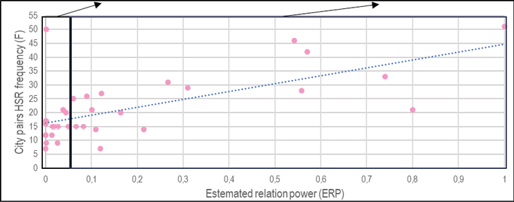
Fig. 7. Estimated relation power verified on operated HSR frequency
Source: European Rail Timetable (2019); own work.
The results from the first part of the paper and the frequency estimation model were synthesised. The correlation between the actual operated HSR frequencies F and estimated HSR frequencies FE differs based on the category of HSR role. As represented in Fig. 8, the correlation value decreases from category A to E as the significance of the HSR role decreases. The correlation value of category A equals R=0.995, category B (R=0.881), category C (R=0.442), category D (R=0.258), and category E (R=0.093). The general correlation value of all HSR routes equals R=0.647.

Fig. 8. Correlation between real operated HSR frequency and HSR frequency estimation model
Source: own work.
In the analysed sample, two extreme values appear, and both belong to category C. The exclusion of extreme values is a standard method of analysed sample normalisation. The first extreme is the route Paris–Lille, where 21 HSR connections are operated, but 64 HSR connections are estimated by the model. The number of estimated connections is strongly influenced by the strength of a relationship and the long operating distance, where HSR dominates compared to conventional trains. The correlation of the category would increase by about 0.157 to R=0.579, and the general value would increase by about 0.055 to R=0.712. The second extreme represents the route Amsterdam–Breda, where 50 HSR connections are operated, but only 9 HSR connections are estimated by the model. The correlation of the category would increase by about 0.272 to R=0.714, and the general value would increase by about 0.133 to 0.780. In total, the category C correlation value would increase to R=0.855 and the general value R=0.852.
This paper challenged the goal to seek a transferable operational experience for countries developing HSR networks based on the currently developed European HSR operational models. That is why the study offers the frequency estimation model formula as a tool for an estimation potentially optimal HSR operational frequency based on the analysis of the sample of 10 European metropolitan regions, more concretely 34 metropolitan core-intermediate city pairs. The paper focuses on a specific segment of HSR network operation: HSR commuting delimited by 1 hour of the operational distance between the metropolitan core and the intermediate city.
The key step to derive the frequency estimation model was to estimate the relation power ERP between the metropolitan cores and intermediate cities, where HSR connections are operated. To reach this estimation the basic gravity model was modified and traditional variables as population, distance, travel time and their variations were used.
The estimated linear relation between the ERP and real operated HSR frequency F on analysed city pairs brought the necessary coefficients to set the formula. It results to Frequency estimation formula FE, which estimates the potential frequency of HSR services on selected relation between metropolitan core and intermediate city delimited by 1h of travel distance.
The potential linear relation between ERP and F based on analysed sample prove the strong correlation R=0.647. In case of extremes elimination, the correlation increases to R=0.852. However, to keep results transparent, the study is presented with extreme values and points to them. The correlation of results variates based on a different role of HSR operation in intermediate cities stations from 0.995 to 0.093 and from that point of view the universal application of Frequency estimation formula without considering the purpose of HSR introduction seems not probable.
The secondary research results bring a partial explanation of such a range of the equation result, which refers to different role of HSR implementation. The supply of rail connections increased substantially by an average of 17%. Above all, however, there was a substantial qualitative change in transport speed. It showed savings of up to 43% in travel time on average, while there were still significant savings of around 25% on the fastest conventional connections. These results are crucial to creating a long-term strategy to motivate people to travel by public transport within a metropolitan area, especially in competition with car transport.
Subjective perceptions of between a quarter and almost a half of the previous travel time play a substantial role in individual decisions about mode choice. This context also raises a follow-up research question that was not the focus of this paper: research on the change in the proportion of travel time by train relative to travel time by car. However, research into historical car travel times from the past century would be somewhat problematic, whereas analysis of train timetables is reasonably reliable in this respect. Of course, the competitive advantage that HSR brings concerning conventional rail and cars is that it frees up existing arterial capacity (on rails, conditional on the parallel operation of conventional and HSR lines). In the case of car transport, substantially higher travel times can be expected in after-peak periods within metropolitan areas precisely because of increasing congestion.
The benefits of HSR relative to existing rail are only sometimes entirely clear in both aspects analysed: frequency and travel time. Therefore, it is always necessary to keep in mind the different starting conditions of each planned HSR project. For this reason, this research presented a typology of five HSR service commuter systems. The categorisation depend on whether the HSR introduced entirely new rail links, brought a complement to existing conventional rail links, created a balanced supply of conventional and HSR links, showed substantial predominance, or marginalised conventional connections (which were more likely to serve even smaller intermediate stops than direct links between the pairs of metropolitan cores under study and their associated intermediate cities).
This typology of identified intra-metropolitan systems of HSR services cannot, by its nature, cover all the institutional, geographical, technical, and socio-economic aspects that influenced the ultimate effectiveness and sensibility of implementing HSR. Only some of the analysed pairs of metropolitan cores and intermediate cities could be strictly classified into the defined categories, as some are typologically located at their imaginary interface. However, this research provides new insights, especially in the somewhat overlooked area of intra-metropolitan transport services within HSR. Indeed, the usual emphasis is on analysing what HSR brings as a link between two or more metropolitan areas, emphasising its impact on the centres of these metropolitan areas. This fact is ultimately the basis for the economic appraisal of HSR planning. However, the analysis of the impact on minor terminals included in the HSR network is a somewhat under-appreciated topic that can make an essential contribution to the possibility of a more comprehensive assessment of the benefits of HSR. Therefore, these findings can also contribute to an accurate assessment of the benefits and costs of future planned developments or projects.
Acknowledgements and funding. This article is the output of the project “New Mobility - High-Speed Transport Systems and Transport-Related Human Behaviour”, Reg. No. CZ.02.1.01/0.0/0.0/16_026/0008430, co-financed by the Operational Programme Research, Development and Education.
ALBALATE, D. and BEL, G. (2012), ‘High‐speed rail: Lessons for policy makers from experiences abroad’,Public Administration Review, 72 (3), pp. 336–349. https://doi.org/10.1111j.1540-6210.2011.02492.x
ANDERSON, J. E. (1979), ‘A theoretical foundation for the gravity equation’, The American Economic Review, 69 (1), pp. 106–116.
BANISTER, D. and BERECHMAN, Y. (2001), ‘Transport investment and the promotion of economic growth’, Journal of Transport Geography, 9, pp. 209–218. https://doi.org/10.1016/S0966-6923(01)00013-8
BARBOSA, F. C. (2018), ‘High speed rail technology: Increased mobility with efficient capacity allocation and improved environmental performance’, [in:] ASME/IEEE Joint Rail Conference (Vol. 50978, p. V001T04A002), American Society of Mechanical Engineers. https://doi.org/10.1115/JRC2018-6137
BERGANTINO, A. S. and MADIO, L. (2020), ‘Intermodal competition and substitution. HSR versus air transport: Understanding the socio-economic determinants of modal choice’, Research in Transportation Economics, 79, 100823. https://doi.org/10.1016/j.retrec.2020.100823
BLUM, U., HAYNES, K. E. and KARLSSON, C. (1997), ‘The regional and urban effects of high-speed trains’, The Annals of Regional Science, 31, pp. 1–20. https://doi.org/10.1007/s001680050036
CAMPOS, J. and de RUS, G. (2009), ‘Some stylized facts about high-speed rail: A review of HSR experiences around the world’, Transport Policy, 16, pp. 19–28. https://doi.org/10.1016/j.tranpol.2009.02.008
CHEN, Ch.-L. and HALL, P. (2012), ‘The wider spatial-economic impacts of high-speed trains – a comparative case study of Manchester and Lille sub-regions’, Journal of Transport Geography, 24, pp. 89–110. doi:10.1016/j.jtrangeo.2011.09.002
CWERNER, S., KESSELRING, S. and URRY, J. (eds) (2009), Aeromobilities., Routledge. https://doi.org/10.4324/9780203930564
ČESKÉ DRÁHY (ČD) (2019), Železničář: Kapacita žekezniční sítě? Na hraně, https://zeleznicar.cd.cz/zeleznicar/tema/kapacita-zeleznicni-site--na-hrane-/-21115/
European Union, (1995-2023), European Statistical System: Census Hub, https://ec.europa.eu/CensusHub2/
GARMENDIA, M., RIBALAYGUA, C. and UREŇA, J. M. (2012a), ‘High speed rail: Implication for cities’, Cities, 29, pp. 526–531. https://doi.org/10.1016/j.cities.2012.06.005
GARMENDIA, M., ROMERO, V., UREŇA, J. M., CORONADO, J. M. and VICKERMAN, R. (2012b), ‘High-speed rail opportunities around metropolitan regions: Madrid and London’, Journal of Infrastructure Systems, 18 (4), pp. 305–313. https://doi.org/10.1061/(ASCE)IS.1943-555X.0000104
GIVONI, M. (2006), ‘Development and impact of the modern high-speed train: A review’, Transport Reviews, 26 (5), pp. 593–611. https://doi.org/10.1080/01441640600589319
GIVONI, M. and DOBRUSZKES, F. (2013), ‘A review of ex-post evidence for mode substitution and induced demand following the introduction of high-speed rail’, Transport Reviews, 33 (6), pp. 720–742. https://doi.org/10.1080/01441647.2013.853707
GUIRAO, B., CAMPA, J. L. and CASADO-SANZ, N. (2018), ‘Labour mobility between cities and metropolitan integration: The role of high speed rail commuting in Spain’, Cities, 78, pp. 140–154. https://doi.org/10.1016/j.cities.2018.02.008
GUIRAO, B., LARA-GALERA, A. and CAMPA, J. L. (2017), ‘High Speed Rail commuting impacts on labour migration: The case of the concentration of metropolis in the Madrid functional area’, Land Use Policy, 66, pp. 131–140. https://doi.org/10.1016/j.landusepol.2017.04.035
GUTIERRÉZ, J., MONZÓN, A. and PIŇERO, J. M. (1998), ‘Accessibility, network efficiency, and transport infrastructure planning’, Environment and Planning A, 30, pp. 1337–1350. https://doi.org/10.1068/a301337
HEUERMANN, D. F. and SCHMIEDER, J. F. (2014), Warping Space: High-Speed Rail and Returns to Scale in Local Labor Markets, Beiträge zur Jahrestagung des Vereins für Socialpolitik 2014: Evidenzbasierte Wirtschaftspolitik, http://hdl.handle.net/10419/100293
L’HOSTIS, A. and BAPTISTE, H. (2006), ‘A transport network for a City network in the Nord-Pas-de-Calais region: linking the performance of the public transport service with the perspectives of a monocentric or a polycentric urban system’, European Journal of Spatial Development, 4 (2), pp. 1–18. https://hal.science/hal-00145683/
LÓPEZ, E., GUTIERRÉZ, J. and GÓMEZ, G. (2008), ‘Measuring regional cohesion effects of large-scale transport infrastructure investments: an accessibility approach’, European Planning Studies, 16 (2), pp. 277–301. https://doi.org/10.1080/09654310701814629
MARTI-HENNEBERG, J. (2013), ‘European integration and national models for railway networks (1840–2010)’,Journal of Transport Geography, 26, pp. 126–138. https://doi.org/10.1016/j.jtrangeo.2012.09.004
MARTI-HENNEBERG, J. (2015), ‘Challenges facing the expansion of the high-speed rail network’, Journal of Transport Geography, 42, pp. 131–133. https://doi.org/10.1016/j.jtrangeo.2015.01.003
MATAS, A., RAYMOND, J. L. and ROIG, J. L. (2020), ‘Evaluating the impacts of HSR stations on the creation of firms’, Transport Policy, 99, pp. 396–404. https://doi.org/10.1016/j.tranpol.2020.09.010
McBRIDE, P. J. (1996), Human geography. Systems, patterns and change, Surrey: Nelson and Sons Ltd.
MD (2017), Ministerstvo dopravy ČR: Strategie: Vysokorychlostní tratě, https://www.mdcr.cz/Dokumenty/Strategie/Vysokorychlostni-trate
MOHÍNO, I., DELAPLACE, M. and UREŇA, J. M. (2018), ‘The influence of metropolitan integration and type of HSR connections on developments around stations. The case of cities within one hour from Madrid and Paris’, International Planning Studies, 24 (2), pp. 156–179. https://doi.org/10.1080/13563475.2018.1524289
MOHÍNO, I., SOLIS, E. and UREŇA, J. M. (2017), ‘Changing commuting patterns in rural metro-adjacent regions: The case of Castilla-La Mancha in the context of Madrid, Spain’, Regional Studies, 51 (7), pp. 1115–1130. https://doi.org/10.1080/00343404.2016.1156238
MONZÓN, A., ORTEGA, E. and LÓPEZ, E. (2013), ‘Efficiency and spatial equity impacts of high-speed rail extensions in urban areas’, Cities, 30, pp. 18–30. https://doi.org/10.1016/j.cities.2011.11.002
MONZÓN, A., ORTEGA, E. and LÓPEZ, E. (2016), ‘Influence of the first and last mile on HSR accessibility levels’, [in:] GEURS, K. T., PATUELLI, R. and DENTINHO, T. P. (eds), Accessibility, Equity and Efficiency, Edward Elgar Publishing, pp. 125–143. https://doi.org/10.4337/9781784717896
MORENO-MONROY, A. I., SCHIAVINA, M. and VENERI, P. (2021), ‘Metropolitan areas in the world. Delineation and population trends’, Journal of Urban Economics, 125, 103242. https://doi.org/10.1016/j.jue.2020.103242
MOYANO, A. (2016), ‘High Speed Rail commuting: Efficiency analysis of the Spanish HSR links’, Transport Research Procedia, 18, pp. 212–219. https://doi.org/10.1016/j.trpro.2016.12.029
MOYANO, A., and DOBRUSZKES, F. (2017), ‘Mind the services! High-speed rail cities bypassed by high speed trains’, Case Studies on Transport Policy, 5 (4), pp. 537–548. https://doi.org/10.1016/j.cstp.2017.07.005
MOYANO, A., RIVAS, A. and CORONADO, J. M. (2019), ‘Business and tourism high-speed rail same-day trips: factors influencing the efficiency of high-speed rail links for Spanish cities’, European Planning Studies, 27 (3), pp. 533–554. https://doi.org/10.1080/09654313.2018.1562657
PERL, A. D. and GOETZ, A. R. (2015), ‘Corridors, hybrids and networks: Three global development strategies for high speed rail’, Journal of Transport Geography, 42, pp. 134–144. https://doi.org/10.1016/j.jtrangeo.2014.07.006
RRG GIS Database (2022), Railway network dataset. RRG Spatial Planning and Geoinformation (RRG). Oldenburg i.H., Germany, www.brrg.de
SPRÁVA ŽELEZNIC (SŽ) (2022), Vysokorychlostní železnice v ČR, https://www.spravazeleznic.cz/vrt
STRASZAK, A. (1977), The Shinkansen high-speed rail network of Japan: Proceedings of an IIASA conference, June 27–30, vol. 7, Elsevier.
TAPIADOR, J. F., BURCKHART, K. and MARTI-HENNEBERG, J. (2009), ‘Characterizing European high speed train stations using intermodal time and entropy metrics’, Transportation Research Part A: Policy and Practice, 43 (2), pp. 197–208. https://doi.org/10.1016/j.tra.2008.10.001
UREŇA, J. M., MENERAULT, P. and GARMENDIA, M. (2009), ‘The high-speed rail challenge for big intermediate cities: A national, regional and local perspective’, Cities, 26 (5), pp. 266–279. https://doi.org/10.1016/j.cities.2009.07.001
UREŇA, J. M., CORONADO, J. M., GARMENDIA, M. and ROMERO, V. (2012), ‘Territorial Implications at National and Regional Scales of High-Speed Rail’, [in:] Territorial Implications of High Speed Rail: A Spanish Perspective, edited by J. M. de Urena, pp. 129–162. Farnham: Ashgate.
VICKERMAN, R. (1997), ‘High-speed rail in Europe: Experience and issues for future development’, The Annals of Regional Science, 31 (1), pp. 21–38. https://doi.org/10.1007/s001680050037
VICKERMAN, R. (2015), ‘High-speed rail and regional development: The case of intermediate stations’, Journal of Transport Geography, 42, pp. 157–165. https://doi.org/10.1016/j.jtrangeo.2014.06.008
VICKERMAN, R., SPIEKERMANN, K. and WEGENER, M. (1999), ‘Accessibility and economic development in Europe’, Regional Studies, 33, pp. 1–15. https://doi.org/10.1080/00343409950118878
VICKERMAN, R. and ULLIED, A. (2009), ‘Indirect and wider economic impacts of high-speed rail’, [in:] de RUS, G. (ed.), Economic Analysis of High-Speed Rail in Europe, Foundation BBVA.