

Abstract. This paper studies spatial differences in the fluctuations of the regional building activity in Greece, by developing a composite multinomial logistic regression model expressing the building activity’s variability in socio-economic terms. The results show that the variability in building activity is related to economies of scale within the construction sector, along with the performance of two other Greek economy’s major sectors, i.e., tourism and tertiary, in highlighting a dependence on the prime drivers of economic and regional development. Overall, the research provides empirical evidence on the macro-economic modelling of spatial demand, based on a proxy incorporating all aspects of human activity in the geographical space.
Key words: spatial planning, regional development, building activity, multinomial logistic regression.
The construction industry is traditionally considered a significant driver of national economies, as well as of regional economic development (Lopes, 2012; Polyzos and Tsiotas, 2020). Construction output typically and consistently contributes worldwide a sizeable proportion, around 7% to 10% of the Gross National Product (GNP), and is responsible for more than half of the national fixed capital generation. It also employs a significant number of the working population, generally between 6% and 8% (Turin, 1973; Wells, 1985; Ball and Wood, 1996; Lopes et al., 2002; Pearce, 2003; Ruddock and Lopes, 2006; Ofori, 2015). Moreover, the construction industry’s products form the main factors of production, such as land and buildings, for almost all the other industrial sectors. Shelter, living accommodation, and transportation are considered the necessities of modern life, and these are provided by construction (Smith and Jaggar, 2007; Polyzos and Tsiotas, 2020). The construction sector is also seen as a major contributor to land use change and, therefore, its role in meeting long-term sustainable development goals is important (Ortiz et al., 2009; Sev, 2009; Lima et al., 2021). Since the building industry mainly delivers fixed long-lasting assets, building production is normally seen, by all parties involved, as a capital investment undertaking (Polyzos, 2019; Zasada et al., 2015). The final product is often large and expensive, and can represent a client’s largest single capital outlay (Ashworth, 2004). The types of building demands are diverse and range from residential buildings, such as houses and blocks of multi-storey apartments, to several types of non-residential building structures, like industrial, commercial, offices, and public buildings of various needs (Seeley, 1996; Polyzos, 2019). Socio-economic development is mainly concerned with expanding the productive capacity of the national economy to increase the quality and extent of goods and services available to the community, or to improve standards of living and economic well-being (Briscoe, 1988; Polyzos, 2019). Thus, apart from its contribution to the total economic flow, the construction industry plays an indispensable role, and the level of building activity is often used as a measure of socio-economic development and progress within a society (Myers, 2008).
Construction activity, as a key sector of overall economic activity, has undoubtedly played an important role in Greece’s development throughout the post-war period (Polyzos and Minetos, 2008; Mavridis and Vatalis, 2015). It has been a key axis around which a significant (if not the most important) part of the country’s economic development has revolved (Polyzos, 2019). The need for recovery and rebuilding on new foundations of the country’s productive apparatus, combined with the need to solve the housing problem for a large percentage of the population, led to a building boom, which functioned autonomously and complementarily to the country’s economic development. Thus, the country’s economic development was largely focused on construction activity and the creation of a productive mechanism that would support it (Polyzos and Minetos, 2008; Mavridis and Vatalis, 2015). The needs for housing were suffocating, especially in Athens, and some estimates put the need for housing across the country in the 1950s and 1960s at 1 million (Polyzos, 2019). In the 1970s, the rate of investment in housing in Greece, which had a long-standing tendency to fall, rose again quite high. Thus, once again, during the then (1970s) crisis, construction filled to some extent the gaps in industrial investment (Polyzos and Minetos, 2008). Already, however, investment in construction was also entering a crisis, based on the data on the volume of new construction, which seems to have been reduced by about half in the Attica region and elsewhere (Polyzos and Minetos, 2008; Mavridis and Vatalis, 2015; Polyzos, 2019). During the 1980s, residential construction was significantly reduced compared to the past, mainly due to a decrease in reconstruction in urban centres. Private and public construction activity experienced a decline in the early 1990s due to the cost of housing. It was affected by high mortgage interest rates, and rising construction costs due to increases in material and labour prices (Polyzos, 2019). However, since the end of 1995, mortgage interest rates have decreased, leases have been liberalised and many areas have been included in the urban plan (Zantanidis and Tsiotras, 1998; Polyzos, 2019). These events together with the 2004 Olympic Games increased construction activity (Polyzos and Minetos, 2008; Polyzos, 2019). Between 1997 and 2005, the number of new houses increased because middle-income earners borrowed to buy housing (Polyzos, 2019). The mortgage system with tax measures led to an increase in housing, especially at the high-quality end. In general, the construction sector experienced a rapid growth from the early 1990s until 2007, significantly increasing its importance in the Greek economy and contributing positively to its growth (Karousos and Vlamis, 2008; Polyzos, 2019; Sdrolias et al., 2022), The positive performance of the sector until recently has been largely due to the absorption of funds for infrastructure projects used under the Community Support Frameworks (CSF), the implementation of Olympic projects, and the growth of private construction activity over time (Polyzos, 2019). Both in the past and today, significant reservations have been expressed about the effectiveness of continued policy support for the construction sector in Greece (Polyzos, 2019), regarding whether this sector of the Greek economy has reached a tipping point or a saturation point, which should lead to the pursuit of different regional development policies.
Within this context, this paper assumes that extending knowledge on the spatial variation in the volume of building activity could assist urban policy decision-makers to identify potential changes in regional economic patterns and alert them to opportunities and risks in markets and regions with differently synchronised economies. To this end, Greece can provide an excellent case for studying building activity as it suggests a country submitted in the last fifty years to considerable urbanisation forces and its modern aspect development is symbiotically related to building activity. The paper has been organised into five sections as follows. Following the introductory section, the second section provides a brief literature review and describes the specific characteristics and territorial dimension of the building activity in Greece, and sets the study area as the spatial unit of analysis. The third section provides a thorough description of the multinomial logistic regression methodology used in the research, the dependent variable, and the explanatory variables that are used in the empirical model. The fourth section presents the analysis results and discusses the spatial configuration of the building activity variance across the Greek prefectures. The paper concludes with a presentation of broader implications and the value of the study to the real estate market and the land use public policy-makers.
The level of building activity represents over time the demand for geographical space due to housing, business, and recreation forces, and suggests a critical driver of both economic growth and regional development. Considering its symbiotic relationship with economic and regional development, further macro-economic evidence on the evolution, spatiality, and current trends in building activity may contribute to a more effective regional policy, planning, and implementation, and provide insights into major questions in regional science as geographic dependency and regional divergence. Ball and Wood (1996) provided evidence of a long-term steady-state relationship between building investment and economic growth for the U.K. from the themed-20th century to the present day. Notwithstanding its significance, fluctuations in building activity output, usually referred to as building or property cycles, are endemic in the industry. In part, they are caused by fluctuations in the economy as a whole and in part by the unique nature of the construction product (Hillebrandt, 2000). Hence, property cycles occur for reasons that are both endogenous (from within the building sector) and exogenous (influences outside the building sector). Endogenous reasons can arise from time lags in production that lead to periods of excess demand and excess supply which means the property market is hardly ever in equilibrium. At first, demand increases but there is a delay before a new building can commence while planning permission and finance are arranged; further shortages of space lead to rising rents bringing forth more new developments; speculation that rents will continue to rise further spurs supply; completions then provide excess supply leading to falling rents and less development. As exogenous influences, they can be considered as any fluctuations in income, employment, availability of credit, interest rates, exchange rates, changes in government policy, etc. A typical example is the introduction of energy performance certificates that posed an additional expense to property owners (Jowsey, 2015). A strong economic upturn coinciding with a shortage of available property may be the starting point of a cycle. Rents and capital values increase, and this can stimulate new development. Further speculative developments are financed by an expansion of bank lending and so a building boom results, but it takes time for supply to reach the market and so rents and capital values continue to rise. When new developments are completed, the business cycle may have peaked and slowed down, causing a fall in demand for property and a property slump with falling values, high vacancy levels, and widespread bankruptcies in the building sector. Undoubtedly, the economy, the property sector, and the financial sector are strongly interlinked (Barras, 1994). According to Towey (2018) and Polyzos (2019), a typical building cycle conceptual model builds on the key characteristics of an economic cycle that are reflected in the building industry, such as a fall/rise in interest rates, a rise/reduction in share prices and value of commodities, and easier/tighter money and rise in property prices, the signs of which are differentiated on the top or bottom of the cycle.
The patterns of these events can affect capital investments that drive or diminish the demand for building activity. Falling interest rates encourage more lending and activity for building work with the opposite in force after a boom. Knowledge of these trends permits building developers and land policy-makers to be aware of the likelihood of changes in demand in both the long and short termsand to implement strategies for future planning. This information aids decision-making around the risks and opportunities available in specific markets to recognise the type of consumer demand that will be in force at given times (Towey, 2018). Although most economic activities are subject to business cycles, the ease with which investment in a building can be postponed makes the difference between the maximum and minimum demand greater than that for most other activities. The greater the amplitude of the fluctuations and their frequency, the less the industry is able to meet future increases in demand as it cannot plan with confidence (Smith and Jaggar, 2007).
Strassmann (1970), as cited in Mehmet and Yorucu (2008), has argued that construction, like agriculture or manufacturing sectors, follows a pattern of change that reflects a country’s level of economic development. After showing a lag in early development, construction accelerates in middle-income countries and then falls rapidly. Goh (2009) studied four countries belonging to the same class of economic development and population, namely Singapore, Finland, Denmark, and Sweden, and concluded that the roles and importance of building activity in the national context could still vary: (i) for a highly developed country with a mature economy, building output volume can be relatively high when the share of construction is relatively low; (ii) the extent to which the government of a country uses the construction industry as an economic regulator is critical in sustaining its importance even when the country is industrially advanced; and (iii) in highly competitive advanced industrialised countries, the building industry can significantly contribute to national competitiveness through a continuous supply of buildings and modernising the country’s physical infrastructure to foster productivity growth and investment.
Regional economies usually experience different periods of either economic growth or decline, and this instability is reflected in higher or lower levels of building activity. These declining, stagnant, or rising patterns of building activity can have a direct effect on regional prosperity level, consumer spending trends, as well as employment opportunities, therefore, providing useful information on the economic performance of a region. Moreover, information on possibly significant spatial variations in regional building activity, within the broader national context, can further contribute considerably to the effectiveness of strategic policy decision-making and implementation (Petrakos and Polyzos, 2005). Exploring variations in the volume produced by the building activity sector can provide useful insights regarding the behaviour of regional property markets and the trajectories of change in the regional land use system. The spatial dimension of building activity variance could add to a clearer understanding of the principal dynamic of increased spatial dependency and regional divergence. The economic underperformance of some regions when compared to others is an indicator of the effectiveness of the applied regional policy (Polyzos and Minetos, 2008). Alkay et al. (2018) emphasised the importance of studying the spatial variation in housing construction activity in Turkey. The authors have suggested that uneven spatial development might be explained in several ways in different parts of the country: in many parts, they have found a reasonable degree of consistency between economic fundamentals and housing activity, but there are exceptions in some regions whereas it seems likely that policy is creating conditions where development levels are outstripping market requirement which, of course, might seek to destabilise the property market and the wider economy; in other regions, development levels may be below what might be required to meet market requirements and to support the growth agenda.
The Building Activity Survey published by the Hellenic Statistical Authority (ELSTAT) has been providing data on a monthly and yearly basis since 1964 (Polyzos, 2019; ELSTAT, 2022). The purpose of this study is to register the total number of building permits issued by the responsible administrative authorities. The survey covers all the features of building activity, such as the type of building permit, the type of construction, the type and the characteristics of a building and its auxiliary spaces, as well as building usage, surface, volume, and value. The survey is fully harmonised with European legislation. The primary legislative act is Regulation (EC) 1165/1998, as it was amended according to Regulation (EC) 1158/2005 and Regulation (EU) No. 2019/2152 of the European Parliament and the Council on European business statistics, as well as Commission Implementing Regulation (EU) No. 2020/1197 laying down specifications and arrangements under Regulation (EU) No. 2019/2152. The survey is exhaustive and covers the total number of issued building permits across the country. The analysis was conducted on the third level of Nomenclature of Territorial Units for Statistics (NUTS-III level), for the fifty-one (51) Greek prefectures, as is shown in Fig. 1.
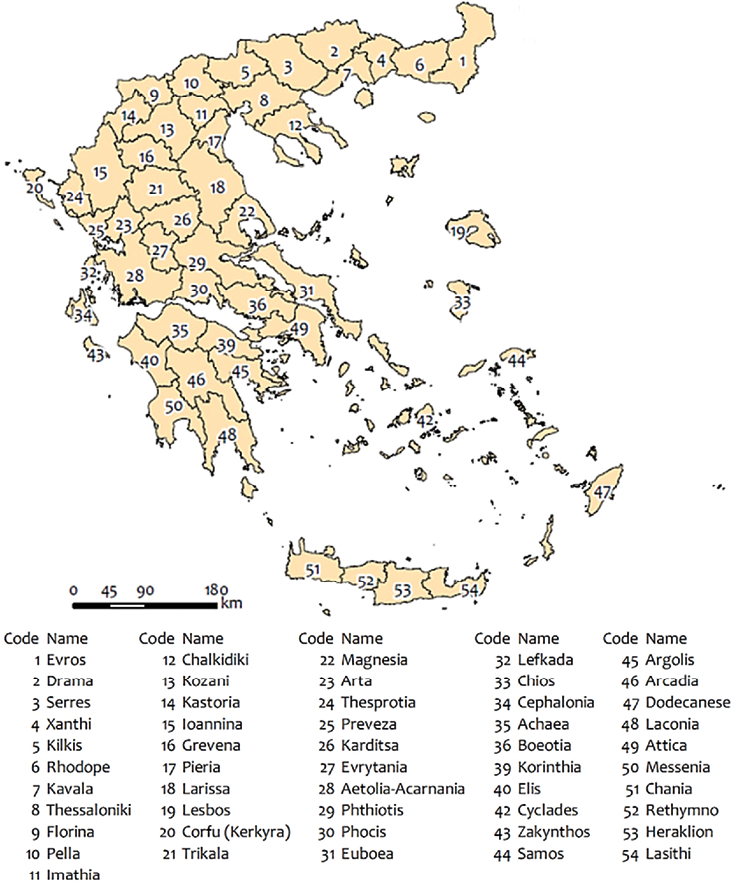
Fig. 1. Map with the 51 prefectures (NUTS-III level) of Greece
Source: own work.
The total building activity for both private and public sectors in Greece is calculated based on the number of issued building permits (Polyzos, 2019; ELSTAT, 2022) and, as of March 2022, amounted to 2,002 permits (ELSTAT, 2022). This amount corresponds to 383,300 sq. m of surface and 1,736,600 cubic m of building volume, reflecting, respectively, a 2.8% increase in the number of building permits, a 19.6% decrease in surface, and a 16.8% decrease in volume, compared with the corresponding month of 2021 (ELSTAT, 2022). The building permits for the private building activity sector issued in March 2022 reached 1,990. This amount corresponds to 382,000 sq. m of surface and 1,731,500 cubic m of volume (ELSTAT, 2022). In comparison with the respective month of 2021, there was a 3.2% increase in the number of building permits, a 15.1% decrease in surface, and a 6% decrease in volume (ELSTAT, 2022). In the same period, from April 2021 until March 2022, private building activity in Greece recorded a 24.4% increase in the number of issued building permits, a 42% increase in the surface, and a 43.2% increase in volume, compared with the corresponding period from April 2020 to March 2021 (ELSTAT, 2022). Based on this information, Fig. 2 shows the fluctuations in the annual private building activity for the period from 2012 to 2021 (expressed as several building permits, surface in sq. m, and volume in cubic m).
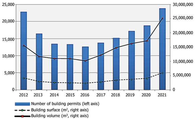
Fig. 2. Annual private building activity in Greece, for the period 2012−2021
Source: own work created on data extracted from ELSTAT (2022).
Next, Fig. 3 shows the fluctuations in monthly private building activity for the period from April 2012 to March 2022, expressed as several building permits, surface in sq. m, and volume in cubic m (ELSTAT, 2022). A building is any permanent and independent structure that has walls and a roof and consists of one or more rooms and other complementary spaces. Building volume refers to the area that is included between the external surface of the external walls, the lowest level (basement or sub-basement, if existent), and the roof of the building. The volume of any open ground floors not enclosed by walls between the lower floor and roof is also considered. The relevant authorities calculate the building volume during the issuing of the building permit. The building surface is the sum of each floor space along with the outer space of the outer walls. A permit refers to all types of building permits: for new buildings or for addition, repair, renovation, demolition, legitimization, amendment, and modification of existing buildings (ELSTAT, 2022).
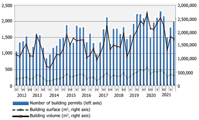
Fig. 3. Monthly private building activity in Greece, for the period Apr 2018−Mar 2022
Source: own work created on data extracted from ELSTAT (2022).
Next, Fig. 4a shows the spatial distribution of the average volume (cubic m) of building activity (per capita) in each Greek prefecture for the period 2000−2019 (NUTS-III level), along with their lower (Fig. 4b) and upper (Fig. 4c) bounds of a 95% confidence interval for the mean. As it can be observed, in the average case (Fig. 4a): the island prefectures of Corfu (20), Cephalonia (28), and Lefkada (34), in the Ionian Sea; the insular Dodecanese (47) and Rethymno, in the Aegean Sea; and the coastal prefecture Achaea (35), in Peloponnese, are described by the lowest volumes of building activity per capita. In terms of spatial distribution, the regions with a very low and low average building activity are located (i) in western Greece (the Ionian Sea prefectures 20, 24, 25, 34, and 43); (ii) in the Peloponnese (including the capital prefecture 35 of the region, along with prefectures 45 and 50); in central and northern Greece (prefectures 13, 14, 16, and 18); in Crete (prefectures 51−53); and in the south and east Aegean (prefectures 44 and 47). Overall, whether the medium (yellow) class regions are also considered, we can observe that regions with below the medium average building activity are scattered throughout the Greek territory, shaping almost an even pattern of dispersion regardless of (insular, coastal, mainland, and mountainous) geomorphology.
On the contrary, the mainland prefectures of Kilkis (5) and Ioannina (15); the coastal metropolitan Attica (49) and Thessaloniki (8); and the island Lasithi (54) have the highest averages of building activity per capita. In terms of spatial distribution, we can observe that the regions with a very high and high average building activity are clustered (i) in north-eastern Greece (prefectures 5, 8, 12, and 7); (ii) in central Greece (prefectures 15, 21, and 26−31); in the metropolitan region of Attica (49); in Laconia prefecture (48) in the Peloponnese; and Lasithi (54), Cyclades (42), and Chios (33), in the Aegean Sea. This arrangement configures a linear spatial pattern described by an arc of a very high and a high average building activity, composed by prefectures 15, 21, 26−31, 33, 42, 49, and 51, ranging from mainland north-western Greece to the insular south Aegean Sea. From both sides of this arc, another cluster of northern Greece prefectures (5, 7, 8, and 12) and the Peloponnese prefecture 48 of low building activity is located. This composite “%-shape” (composed of the central arc and clusters from both sides) spatial pattern of a high average building activity appears to be an effect of demographic concentration (to the extent the metropolitan regions of the country are concerned), tourism development (as far as tourism developed insular and coastal prefectures is concerned), and mainland geomorphology related to a high specialisation in the primary sector. To the extent that the building activity is related to regional development, we can observe that the potential drivers of this spatial configuration are the major drivers (population, tourism, and agriculture) stimulating regional development in Greece (Polyzos, 2019; Tsiotas, 2021; Tsiotas et al., 2021; Kranioti et al., 2022). This observation can also drive the selection of the covariates in the regression models.
Furthermore, as far as metropolitan regions are concerned, we can observe that (i) two (31 and 42) out of four (50%) neighbour prefectures (31, 36, 39, and 42) of Attica (49) have a high building activity; whereas (ii) two (5 and 12) out of six (30%) neighbour prefectures (3, 5, 10−12, and 17) of Thessaloniki (8) have a high building activity. In the context of the growth pole theory (Capello, 2016; Polyzos, 2019; Tsiotas et al., 2022), this observation enables one to configure a composite model of the corporate neighbourhood between the metropolitan and satellite regions in Greece in terms of building activity, according to which there seems to be a “selective” diffusion of building activity from the metropolitan regions to their satellites, of an intensity almost proportional to the metropolitan regions’ population density. This observation addresses the avenues of further research. Finally, we can observe that, in the majority of cases, Fig. 4b and Fig. 4c illustrate the same patterns as the average cases, except the prefectures of (i) Kozani (13), which climbs (2→3) a class in building activity at the upper bound case (Fig. 4b,c); (ii) Pieria (17), which climbs and falls (2→3→2) one class in building activity across cases (Fig. 4a,b); (iii) Thesprotia (24), which climbs and falls (2→3→2) one class in building activity across cases (Fig. 4a,b,c); (iv) Karditsa (26), which climbs (4→5) a class in building activity at the upper bound case (Fig. 4b,c); (v) Evrytania (27), which falls and climbs (4→3→4) one class in building activity during cases (Fig. 4a,b,c); (vi) Boeotia (36), which climbs (2→3) a class in building activity at the upper bound case (Fig. 4b,c); and (vii) Rethymno (36), which climbs (1→2) a class in building activity at the upper bound case (Fig. 4b,c). These “commuting” cases in classification can be of particular interest in terms of regional policy as they appear the most “sensitive” in transitions between classes of building activities, and, therefore, the measures of regional policy motivating building activity can be more effective by dint of their “sensitivity”.
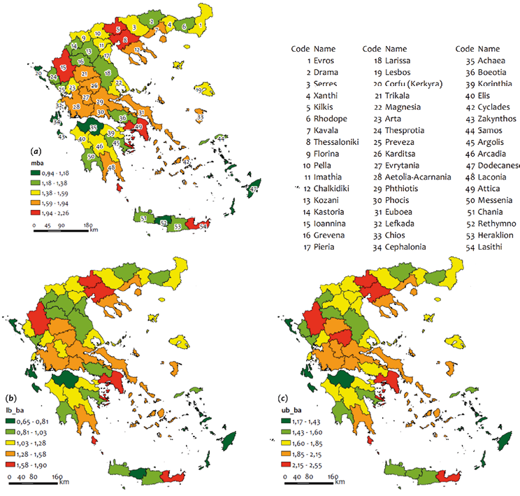
Fig. 4. Spatial distribution of (in cubic m) of building activity’s volume per capita by Greek prefectures expressed in (a) average values of building activity (mba); (b) lower bound of a 95% confidence interval (lb_ba); and (c) upper bound of a 95% confidence interval (lb_ba). Data of the period 2000-2019
Source: own work.
Finally, Fig. 5 shows the volume (in cubic m) of private building activity in the Greek regions (NUTS-II level) for the years 2021−2022. As of March 2022, the cases of Attiki (region 10), Kentriki Makedonia (Central Macedonia, 02), and the Peloponnisos (Peloponnese, 09) were the leading regions in building activity whilst the cases of Voreio Aigaio (North Aegean, 11), Dytiki Makedonia (West Macedonia, 03), and Sterea Ellada (Sterea Hellas, 08) showed the lowest building volume levels (ELSTAT, 2022). Further, the number of firms operating broadly in the Greek construction sector reached 158,305 in 2019, representing a decline of 11.2% since 2010. In contrast, the real estate and architectural/engineering sub-sectors reported in 2019 a 50.5% and a 21.3% increase in the number of firms, respectively, compared to the levels in 2010. In terms of employment, the number of individuals employed in the broad construction sector stood at 280,280 in 2019, representing a decline of 25.8% since 2010. Conversely, the number of persons employed in the property and architectural/engineering activities sub-sectors increased by 46.0% and 26.7% from 2010 to 2019, respectively (ECSO, 2020).
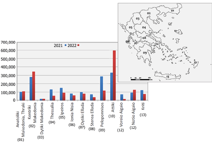
Fig. 5. Private building activity (in cubic m) by Greek regions (2021−2022)
Source: own work created on data extracted from ELSTAT (2022).
This study aims at exploring significant socio-economic factors that affected Greek building activity. The analysis builds on a multinomial logistic approach applied at the third (III) level of spatial administration, according to the Nomenclature of Territorial Units for Statistics (NUTS). The dependent variable represents the variance in building activity (vba) for the study period, as reported by the Hellenic Statistical Authority (ELSTAT, 2022) for the fifty-one (51) Greek prefectures (see Fig. 1). In particular, the dependent variable expresses the variance in the volume (in cubic m) of building activity per capita in each prefecture and is allocated to low, medium, high or very high levels. Due to the data availability of the independent variables, a list-wise analysis restricts the availability of the respective building activity’s data (as shown in Fig. 2 and Fig. 3) to the period 2000−2019. To repair this loss of information, a composite multinomial logistic regression has been used, consisting of a collection of three models conceived in a statistical inference context based on a confidence interval computation. In particular, three multinomial logistic regression models were constructed including collections of (i) lower bound, (ii) average, and (iii) upper bound variables, and, therefore, the analysis was run three times (instead of once) to incorporate in the results a 95% certainty level captured by the confidence intervals computed across the time dimension (2000−2019) of the available variables. In the final step, this approach enables one to consider in common the results of the analysis based on signs’ intersection and, therefore, to repair and better manage the uncertainty caused by the definition of the period 2000−2019.
The total surface area of Greece is 132,049 sq. km (Polyzos, 2019; Tsiotas, 2021) with Kentriki Makedonia representing the biggest region (19,166 sq. km) and the Ionian Islands the smallest one (2,306 sq. km). According to the 2011 Population – Housing Census, the total population of Greece was 10,816,286 residents. The prefecture of Attiki (1) has the greatest regional population with 3,828,434 residents (35.4% of the country’s population) and the lowest population with 199,231 residents (only 1.8% of the country’s population) has the Voreio Aigaio (11) region. The total number of households reaches 4,134,540, with 2-membered ones representing 29.5% (1,218,466 households). Furthermore, according to the 2016 Farm Structure Survey, the total utilised agricultural area in Greece is 3.1526 thousand ha. The independent variables which are considered in the analysis regard economic and social regional characteristics.
All models in this paper were constructed through the use of the IBM SPSS® statistical package (Norusis, 2011). Next, a description of the methodology adopted is provided and the composite model’s structure is explained in more detail.
The spatial effect of the observed differences in building activity variance can be described by a categorical variable that assigns spatial ranges to a specific number of categories concerning the magnitude of variance so that the dimensions of the phenomenon under study can be reduced and sustain only its major trends in variance. The result contributes to a clearer and more intuitive understanding of any spatial dissimilarity (Polyzos and Minetos, 2008). For this presented analysis, a set of three multinomial logistic regression (MLR) models is used (Norusis, 2011), described by four classes (dimensions) of building activity variance. The MLR is useful when there is a need to classify subjects based on the values of a set of predictor variables. This type of regression is like a logistic regression, but the dependent variable is not restricted to two categories. Logistic regression treats the distribution in a probabilistic manner and expresses each dimension of the issue under investigation in terms of probability (Agresti, 1996). The MLR technique is an extension of the binomial logistic model to the cases where the dependent variable has more than two categories (e.g., low variance, medium variance, high variance, etc.). In this case, the dependent variable of interest exhibits a multinomial distribution and not a binomial as in simple logistic modelling. This type of regression requires no linear relationship between the dependent and independent variables to apply. Furthermore, it does not assume that the dependent variable and residuals are normally distributed (Norusis, 2011). The “very high variance” category (cat) is set as a reference category, and three non-redundant classes (logits) are formed for (i) the “high variance”; (ii) “medium variance”; and (iii) “low variance” categories, to observe differences in building activity variance. Using the general formula of logistic regression (Norusis, 2011):
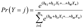 | (1) |
which is equivalent to:
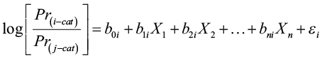 | (2) |
the following logits can be constructed for a single model:
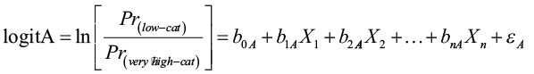 | (3) |
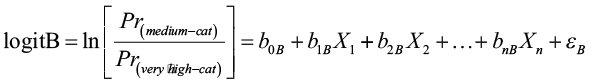 | (4) |
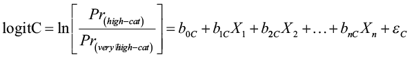 | (5) |
where:
Y: the dependent categorical variable
j: the baseline category (j-cat)
i: the alternative (different than the baseline) categories (i-cat), numbered 1, …, m
Pr(j-cat): the likelihood that the dependent categorical variable Y is in the j category (j-cat)
Pr(i-cat): the likelihood that the dependent categorical variable Y is in the i category (i-cat)
Xn: the independent variables (predictors), numbered as 1, …, n
b0i: the intercept for logit i
b1i ~ bni: the regression coefficients of the n independent variables (predictors) for logit i
εi: the error terms (residuals) for logit i.
Logit A captures the log of the odds of the probability that a prefecture is in the “low building activity variance” category rather than in the very high category. Logit B incorporates the log of the odds of the probability of being in the “medium building activity variance” category compared to the very high variance category. Logit C captures the log of the odds of the probability that a prefecture is in the “high building activity variance” category rather than in the very high category. The MLR’s main output result is the logistic coefficient (B) for each predictor variable, for each alternative category (not the reference category) of the outcome variable. This B coefficient is the expected amount of change in the logit for each one-unit change in the predictor variable. The logit is what is being predicted, namely, it is the odds of being in the category of the outcome variable which has been specified. The closer B coefficient is to zero, the less influence the predictor has in predicting the logit. The results also entail the standard error, t-statistic, and p-value. The t-test for each coefficient is used to determine whether the coefficient is significantly different from zero. The Pseudo R-Square statistics (e.g., McFadden) are treated as measures of effect size, like how R² is treated in standard multiple regression. However, these types of metrics do not always represent the amount of variance in the outcome variable accounted for by predictor variables. Higher values generally indicate a better fit, but they should be interpreted with caution. The likelihood ratio chi-square test is the alternative test of goodness-of-fit. The use of the MLR and relevant discussion can be found in Hosmer and Lemeshow (1989), Long (1997), and Menard (2000).
Data for estimating regional differences in building activity was extracted from the Hellenic Statistical Authority (ELSTAT). The dependent variables (vba) are estimations of the variance (σ2) in the building activity within each Greek prefecture (NUTS-III level) for the years 2000−2019, expressed in volume (cubic m) per capita. In particular, the first dependent variable Y1 ≡ vba(LB) expresses the lower bound of the average variance in building activity, estimated by a 95% confidence interval that is computed (based on Student’s distribution) across the available time data (2000−2019) for each prefecture. The second dependent variable Y2 ≡ vba(M) expresses the average variance in building activity, estimated (point estimation) across the available time data for each prefecture. The third dependent variable Y3 ≡ vba(UB) expresses the upper bound of the average variance in building activity, estimated by a 95% confidence interval that is computed (again based on Student’s distribution) across the available time data (2000−2019) for each prefecture. The collection of these three models Y={Y1, Y2, Y3,} is implemented to repair uncertainty due to the data availability, and is expressed in a system format as follows:
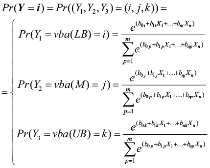 | (6) |
All these latent variables were derived from the mean values (see Fig. 3) and the standard deviation of building activity volume divided by the population of each prefecture. These original values of variances were transformed to construct a broader variance classification of building activity and subsequently to investigate the relative performance of the building sector against a diverse group of numerical variables considered hereinafter as significant driving factors of building activity fluctuations. Hence, the 51 prefectures were classified into four categories according to the magnitudes of variance that they exhibited during the study period. These categories (cat) are equally weighted and, indicatively for the second model (Y2), are shown as follows:
cat(1): Prefectures with low variance in building activity (vba(MB) ≤ 4.27)
cat(2): Prefectures with medium variance in building activity (4.27 < vba(MB) ≤ 6.45)
cat(3): Prefectures with high variance in building activity (6.45 < vba(MB) ≤ 9.76)
cat(4): Prefectures with very high variance in building activity (9.76 < vba(MB))
The corresponding categories for the other two models (Y1 and Y2) arise from the previous ones by the confidence intervals calculation.
This section presents the total eight independent variables (predictors) selected to be included in the empirical model together with the main research hypothesis assigned to each variable. The relevant data was retrieved from ELSTAT databases and covers the study period of the years 2000−2019. These explanatory variables are considered to be related to several economic and social regional characteristics and are shown in Table 1. As far as the pre-variable is concerned (prefecture’s GDP to the GNP), according to Myers (2008), GDP figures are used worldwide as a proxy for a territory’s progress towards prosperity. Since “the more money made,” the higher the GDP growth, it is generally accepted that an increased GDP is associated with a higher standard of living for the citizens of that territory.
| Label | Name | Description | Source |
|---|---|---|---|
| pre | Prefecture’s gross domestic product (GDP) contribution to the gross national product (GNP) | Represents the prosperity level of residents in each prefecture and is used to investigate whether there is a positive influence of the level of economic development in each prefecture on the variance of building activity (expressed as a percentage). | Polyzos (2019); Tsiotas (2021) |
| dic | The declared income per resident in each prefecture | It also relates to residents’ prosperity level in each prefecture and is used to explore whether there is a positive effect of higher declared income in each prefecture on the building activity variance (expressed as euro per capita). | Polyzos (2019); Tsiotas (2021) |
| pit | Personal income tax in each prefecture | It examines whether there is a negative relationship between higher levels of taxation on personal income and the variance of building activity in each prefecture (expressed as euro per capita). | Polyzos (2019) |
| upd | Urban population density | It measures the level of urbanisation of each prefecture; due to the phenomenon of real estate cycles, the relationship between the growth of urban population and the level of building activity is rather a complex one and, therefore, the hypothesis under investigation is whether prefectures with larger urban concentrations are associated with more stable patterns of building activity.
The extent of building activity in an economy is closely linked in particular to the extent of urbanization in that economy (expressed as the number of residents per sq. km of each prefecture’s surface area). |
Tsiotas (2021) |
| con | Construction industry’s contribution to each prefecture’s GDP | It is used to assess whether increased levels of construction activity within a prefecture could be associated with more volatile building activity levels (expressed as a percentage). | Polyzos (2019) |
| agr | Agricultural sector’s contribution to each prefecture’s GDP | It is used to check whether the growth of agricultural activity within a prefecture could be associated with higher levels of building activity variance (expressed as a percentage). | Tsiotas (2021); Sdrolias et al. (2022) |
| srv | Services sector’s contribution to each prefecture’s GDP | It is used to check whether an increased level of activities related to the services industry within a prefecture could be associated with more unstable building activity patterns (expressed as a percentage). | Tsiotas (2021) |
| toa | Tourists’ overnight accommodation | It captures the magnitude of touristic demand for each prefecture and, thus, it is investigated whether higher demand for tourists’ overnight staying is connected to an increased level of building activity variance (expressed as the number of nights spent by tourists in each prefecture per capita of that prefecture). | Tsiotas et al. (2021) |
Table 2a reports no missing values for the binned categorical (ordinal) dependent variables (vba(LB), vba(M), vba(UB)). Table 2b presents Models Fitting Information with the Likelihood Ratio Test (Chi-Square), used to test the hypothesis that the values for all coefficients in the multinomial logistic model are zero. Since the observed level of significance is asymptotically zero, the null hypothesis that all coefficients for the independent variables are zero can be rejected in all cases of the three models. Thus, it is concluded that the final models outperform the intercept-only models. The null hypothesis that the models adequately fit the data can be examined by the Deviance Goodness-of-Fit test results shown in Table 2c. However, in the cross-tabulation, there are 153 (75%) cells (i.e., dependent variable levels by subpopulations) with zero frequencies due to a large number of regressors in the model (eight covariates). Therefore, it is advisable not to rely on the above tests. Pseudo R-Square statistics (Table 2d) are measures capturing the goodness-of-fit of the model, to the extent that (Pseudo R-Square) values closer to 1 show that the logistic model explains well the variation in the dependent variable. The Cox and Snell and Nagelkerke scores can be considered satisfactory (Nagelkerke, 1991) for all three models, although we can observe that they slightly decline across models configuring an inequality R2(vba(LB)) > R2(vba(M)) > R2(vba(UB)).
| Model (Dependent variable) |
vba(LB) (Lower bound) |
vba(M) (Mean) |
vba(UB) (Upper bound) |
||||
|---|---|---|---|---|---|---|---|
| Descriptives | N | Marginal Percentage | N | Marginal Percentage | N | Marginal Percentage | |
| Categories | (1) | 39* | 76.5%* | 39* | 76.5%* | 39* | 76.5%* |
| (2) | |||||||
| (3) | |||||||
| (4) | 12 | 23.5% | 12 | 23.5% | 12 | 23.5% | |
| Valid | 51 | 100.0% | 51 | 100.0% | 51 | 100.0% | |
| Missing | 0 | ||||||
| Total | 51 | ||||||
| Subpopulation | 51* | ||||||
| Model | Model Fitting Criteria | Likelihood Ratio Tests | ||
|---|---|---|---|---|
| -2 Log Likelihood | Chi-Square | df | Sig. | |
| Model: vba(LB) | ||||
| Intercept Only | 141.342 | |||
| Final | 70.843 | 70.500 | 24 | .000 |
| Model: vba(M) | ||||
| Intercept Only | 141.342 | |||
| Final | 79.051 | 62.291 | 24 | .000 |
| Model: vba(UB) | ||||
| Intercept Only | 141.342 | |||
| Final | 83.138 | 58.204 | 24 | .000 |
| Type | Chi-Square | df | Sig. |
|---|---|---|---|
| Model: vba(LB) | |||
| Pearson | 88.040 | 126 | .996 |
| Deviance | 70.843 | 126 | 1 |
| Model: vba(M) | |||
| Pearson | 95.204 | 126 | .981 |
| Deviance | 79.051 | 126 | 1 |
| Model: vba(UB) | |||
| Pearson | 100.791 | 126 | .952 |
| Deviance | 83.138 | 126 | .999 |
| ↓Statistic / Model→ | vba(LB) | vba(M) | vba(UB) |
|---|---|---|---|
| Cox and Snell | .749 | .705 | .681 |
| Nagelkerke | .799 | .752 | .726 |
| McFadden | .499 | .441 | .412 |
The Likelihood Ratio Tests that are reported in Table 3 evaluate the contribution of each effect to the corresponding model. Thus, each coefficient is tested and the hypothesis that each coefficient is zero is examined. The -2 Log-likelihood is computed for each effect for the reduced model, i.e., a model without the effect. In cases where the significance of the test is small (less than 0.05 or 0.10), the effect contributes to the corresponding model. This test can be used instead of the Wald test for the parameter estimates. As it can be observed, five (pre, pit, con, agr, toa) out of the total eight covariates make a significant contribution to the lower bound model (Y1 = vba(LB)); another five (pit, con, agr, srv, toa) covariates (62.5% of the total) make a significant contribution to the average vba model (Y1 = vba(LB)); whereas four (pit, con, srv, toa) covariates (50% of the total) make a significant contribution to the lower bound model (Y1 = vba(LB)). Amongst these covariates, pit, con, and toa are in common in all these three models; covariates agr and srv appear significant in two out of three models, whereas covariate pre appears significant in a single model. This observation enables one to put into a hierarchy the contribution of the covariates to the model as follows whether multiplying their significances for all three models and concluding to the following ranking: con (average significance: ≤0.001), pit (average significance: 0.043), toa (average significance: 0.045), agr (average significance: 0.07), srv (average significance: 0.157), and pre (average significance: 0.392), where the first four in ranking covariates are on average significant (≤0.01).
The Classification matrix in Table 4 shows that the models on average perform satisfactorily (>60.0%) in identifying the prefectures that experience high (class 4) low (class 2) and very high (class 5) variances in building activity. Overall, for all three models, more than 60% of the predictions have been classified correctly. Although this percentage cannot be claimed as an uncontested high one, it can be considered satisfactory to the extent that the models’ results are interpreted structurally, namely based on their significance (to differ from zero) and their (positive or negative) sign indicating the analogy of their contribution to the model. Towards this direction, the construction of a composite (three-layer) model, based on the confidence interval estimations of the available dependent and independent variables, contributes to the increase of our structural certainty about the relationship vba=f(pre, dic, pit, upd, con, agr, srv, toa). Within this context, being aware of such limitations, we focus on the sign interpretations of the model results and not on their detailed numeric values.
The results of parameter estimates for the three logits A, B, and C and per model (vba(LB), vba(M), vba(UB)) are shown in Table 5, which summarises the effect of each independent variable. Predictors that significantly contribute to the separation of low, medium, and high building activity variance categories from the very high variance reference category are highlighted (see variables and associated values) in bold font, whereas those of marginal contribution is shown in italics. In general, parameters with negative coefficients decrease the likelihood of that response category for the reference category. Conversely, parameters with positive coefficients increase the likelihood of the response category concerning the reference one.
| Model | vba(LB) | vba(M) | vba(UB) | |||||||||
|---|---|---|---|---|---|---|---|---|---|---|---|---|
| Effect | Fitting Criteria | Likelihood Ratio Tests | Fitting Criteria | Likelihood Ratio Tests | Fitting Criteria | Likelihood Ratio Tests | ||||||
| -2 Log Likelihood of Reduced** Model | x2 (***) | df | Sig. | -2 LL of Reduced Model | x2 | df | Sig. | -2 LL of Reduced Model | x2 | df | Sig. | |
| Intercept | 78.639 | 7.796 | 3 | .050 | 90.109 | 11.058 | 3 | .011 | 93.277 | 10.139 | 3 | .017 |
| pre | 80.411 | 9.568 | 3 | .023 | 81.322 | 2.270 | 3 | .518 | 84.843 | 1.706 | 3 | .636 |
| dic | 75.849 | 5.006 | 3 | .171 | 80.816 | 1.764 | 3 | .623 | 84.366 | 1.228 | 3 | .746 |
| pit | 81.946 | 11.103 | 3 | .011 | 86.045 | 6.994 | 3 | .072 | 91.077 | 7.939 | 3 | .047 |
| upd | 75.959 | 5.116 | 3 | .163 | 80.213 | 1.161 | 3 | .762 | 83.791 | .653 | 3 | .884 |
| con | 86.221 | 15.379 | 3 | .002 | 97.495 | 18.444 | 3 | .000 | 100.475 | 17.337 | 3 | .001 |
| agr | 78.039 | 7.196 | 3 | .066 | 87.434 | 8.382 | 3 | .039 | 89.305 | 6.167 | 3 | .104 |
| srv | 74.090 | 3.247 | 3 | .355 | 86.284 | 7.233 | 3 | .065 | 90.935 | 7.797 | 3 | .050 |
| toa | 78.765 | 7.922 | 3 | .048 | 87.987 | 8.936 | 3 | .030 | 90.667 | 7.529 | 3 | .057 |
|
* The null hypothesis is that all parameters of that effect are 0 ** The reduced model is formed by omitting an effect from the final model *** The chi-square statistic is the difference in -2 log-likelihoods between the final model and a reduced model |
||||||||||||
| Observed | Predicted | ||||
|---|---|---|---|---|---|
| cat (1) | cat (2) | cat (3) | cat (4) | Percent Correct | |
| Model: vba(LB) | |||||
| cat (1) | 8 | 3 | 1 | 1 | 61.5% |
| cat (2) | 3 | 7 | 3 | 0 | 53.8% |
| cat (3) | 1 | 1 | 9 | 2 | 69.2% |
| cat (4) | 1 | 1 | 2 | 8 | 66.7% |
| Overall Percentage | 25.5% | 23.5% | 29.4% | 21.6% | 62.7% |
| Model: vba(M) | |||||
| cat (1) | 7 | 3 | 2 | 1 | 53.8% |
| cat (2) | 2 | 10 | 0 | 1 | 76.9% |
| cat (3) | 4 | 1 | 6 | 2 | 46.2% |
| cat (4) | 1 | 0 | 3 | 8 | 66.7% |
| Overall Percentage | 27.5% | 27.5% | 21.6% | 23.5% | 60.8% |
| Model: vba(UB) | |||||
| cat (1) | 7 | 3 | 2 | 1 | 53.8% |
| cat (2) | 4 | 7 | 2 | 0 | 53.8% |
| cat (3) | 3 | 1 | 7 | 2 | 53.8% |
| cat (4) | 1 | 0 | 3 | 8 | 66.7% |
| Overall Percentage | 29.4% | 21.6% | 27.5% | 21.6% | 56.9% |
For the first logit A grouping (low variance), significant variables across all three vba models are the size of the construction sector (con) and the tourists’ overnight accommodation (toa), whereas the size of the agricultural sector (agr) is significant in one model, and the share of the services to the total GDP of each prefecture (srv) appear marginally significant in two out of three models. Next, for the second logit B grouping (medium variance), the size of the construction sector (con) remains a significant covariate across all three models, whereas the number of tourists overnight accommodation (toa) appears significant in two out of three models and in one marginally significant. Further, the share of the services sector to the prefecture’s GDP (srv) appears this time significant in two out of three models, and the prefecture’s contribution to total GNP (pre) in one out of three models. Next, according to the third logit C grouping (high variance), the personal income tax (pit), the share of the services sector to the prefecture’s GDP (srv), and the number of tourists’ overnight accommodation (toa) can be considered marginally significant in one out of three models.
| Type | vba(LB) | vba(M) | vba(UB) | |||||||||||||
|---|---|---|---|---|---|---|---|---|---|---|---|---|---|---|---|---|
| b | s.e. | Wald | Sig. | eb | b | s.e. | Wald | Sig. | eb | b | s.e. | Wald | Sig. | eb | ||
| cat (1) | Intercept | 76.584 | 63.954 | 1.434 | .231 | 32.954 | 33.519 | .967 | .326 | 34.863 | 31.198 | 1.249 | .264 | |||
| logit A | pre | -.541 | 2.074 | .068 | .794 | .582 | -1.478 | 1.761 | .704 | .401 | .228 | -1.322 | 1.749 | .572 | .450 | .266 |
| dic | -6.475 | 6.913 | .877 | .349 | .002 | .647 | 2.090 | .096 | .757 | 1.909 | .477 | 1.560 | .094 | .760 | 1.612 | |
| pit | -1.527 | 10.271 | .022 | .882 | .217 | -6.888 | 9.549 | .520 | .471 | .001 | -8.952 | 9.723 | .848 | .357 | .000 | |
| upd | -.694 | 2.151 | .104 | .747 | .499 | -.445 | 1.768 | .063 | .801 | .641 | -.002 | 1.732 | .000 | .999 | .998 | |
| con | -11.926b | 5.162 | 5.338 | .021 | <0.001 | -12.776 | 4.836 | 6.980 | .008 | <0.001 | -11.089 | 4.301 | 6.647 | .010 | <0.001 | |
| agr | -2.381 | 2.617 | .828 | .363 | .092 | -2.721 | 2.270 | 1.437 | .231 | .066 | -2.682 | 2.170 | 1.527 | .217 | .068 | |
| srv | 5.634 | 3.841 | 2.152 | .142 | 279.887 | 4.325 | 3.369 | 1.648 | .199 | 75.548 | 4.707 | 2.996 | 2.469 | .116 | 110.747 | |
| toa | -2.303 | 1.025 | 5.047 | .025 | .100 | -2.235 | .913 | 5.999 | .014 | .107 | -1.946 | .912 | 4.557 | .033 | .143 | |
| cat (2) | Intercept | -17.932 | 28.055 | .409 | .523 | -8.980 | 29.737 | .091 | .763 | -5.721 | 29.854 | .037 | .848 | |||
| logit B | pre | -4.901 | 2.278 | 4.629 | .031 | .007 | -2.563 | 1.832 | 1.957 | .162 | .077 | -2.143 | 1.760 | 1.482 | .223 | .117 |
| dic | -.963 | 2.074 | .215 | .643 | .382 | 1.313 | 1.179 | 1.240 | .265 | 3.718 | .980 | 1.127 | .756 | .385 | 2.663 | |
| pit | 14.848 | 11.080 | 1.796 | .180 | 2.81∙106 | 3.000 | 9.790 | .094 | .759 | 20.095 | 3.911 | 9.921 | .155 | .693 | 49.930 | |
| upd | 2.904 | 2.345 | 1.534 | .216 | 18.246 | .886 | 1.801 | .242 | .623 | 2.426 | .971 | 1.766 | .302 | .582 | 2.640 | |
| con | -13.293 | 5.285 | 6.326 | .012 | <0.001 | -13.765 | 4.944 | 7.750 | .005 | <0.001 | -12.298 | 4.356 | 7.971 | .005 | <0.001 | |
| agr | 2.588 | 2.576 | 1.009 | .315 | 13.307 | 1.350 | 2.241 | .363 | .547 | 3.856 | .326 | 2.186 | .022 | .881 | 1.386 | |
| srv | 4.402 | 3.678 | 1.432 | .231 | 81.619 | 6.701 | 3.353 | 3.994 | .046 | 813.574 | 6.114 | 2.992 | 4.176 | .041 | 452.239 | |
| toa | -1.677 | .944 | 3.158 | .076 | .187 | -1.476 | .905 | 2.661 | .103 | .229 | -1.761 | .877 | 4.030 | .045 | .172 | |
| cat (3) | Intercept | 53.664 | 57.123 | .883 | .347 | -27.674 | 26.834 | 1.064 | .302 | -21.838 | 26.503 | .679 | .410 | |||
| logit C | pre | -1.201 | 1.697 | .501 | .479 | .301 | -1.012 | 1.420 | .507 | .476 | .364 | -.761 | 1.349 | .318 | .573 | .467 |
| dic | -10.069 | 7.083 | 2.020 | .155 | <0.001 | .784 | 1.025 | .585 | .444 | 2.190 | .684 | .981 | .485 | .486 | 1.981 | |
|
logit C
|
pit | 15.509 | 10.518 | 2.174 | .140 | 5.44∙106 | 8.908 | 8.996 | .980 | .322 | 7390.986 | 7.246 | 9.066 | .639 | .424 | 1402.527 |
| upd | .898 | 1.845 | .237 | .626 | 2.456 | .560 | 1.575 | .126 | .722 | 1.750 | .487 | 1.535 | .101 | .751 | 1.627 | |
| con | -4.046 | 4.479 | .816 | .366 | .017 | -3.274 | 3.677 | .793 | .373 | .038 | -3.337 | 3.263 | 1.046 | .306 | .036 | |
| agr | .484 | 2.226 | .047 | .828 | 1.622 | .779 | 1.837 | .180 | .672 | 2.178 | .479 | 1.764 | .074 | .786 | 1.615 | |
| srv | 4.530 | 3.247 | 1.946 | .163 | 92.750 | 4.122 | 2.763 | 2.225 | .136 | 61.658 | 3.577 | 2.534 | 1.991 | .158 | 35.750 | |
| toa | -1.091 | .761 | 2.058 | .151 | .336 | -.849 | .631 | 1.812 | .178 | .428 | -.798 | .610 | 1.710 | .191 | .450 | |
By multiplying the significances per covariate, for all 9 cases composed by the multiplication of 3 vba models and 2 logit categories, it can be observed in Table 6 that (i) those covariates that remain significant at the 0.10 level (≤0.109) are the size of the construction sector (con) and the number of tourists overnight accommodation (toa); (ii) the covariate that remains marginally significant at the 0.12 level (≤0.129) is the share of the services sector to the prefecture’s GDP (srv); whereas (iii) the fourth covariate in the ranking, the prefecture’s contribution to total GNP (pre), has a product of significance >0.309 and cannot be considered as significant along with its following ones.
As far as the significant predictors are concerned, the size of the construction sector (con) appears the most significant one, having a negative coefficient in all cases that absolutely increases and afterward decreases across the logit groups (in an inverse U-shaped pattern). This outcome first indicates that the size of building activity in a prefecture (as it represents a major constituent of its total construction volume) is positively associated with its variance. This observation, in the context of the Williamsons’ curve of inequalities, which describes an inverse U-shaped engine between economic national economic growth and regional inequalities (Capello, 2016; Polyzos, 2019), enables one to assume (by loosely assigning the size of the construction sector to the economic growth’s axis and the variability of building activity to the regional inequalities’ axis) a similar engine describing the vba’s distribution by the size of the construction sector, interpreting that as the size of the construction section increases (from low to high) the variability in the sector first increases and afterward decreases. This interpretation may imply that intermediate stages of growth in the construction sector appear more unevenly distributing the returns of growth in the structural elements of the spatial economic system (e.g., a prefecture), whereas the cases of low and high size in the construction sector appear more convergent, addressing avenues of further research for testing this hypothesis.
Next, the second most significant predictor is the number of tourists overnight accommodation (toa), showing also a negative coefficient across all cases, which, however, absolutely decreases across the logit groups. This outcome supports the hypothesis that prefectures with an increased touristic demand are more likely to experience high levels of variance in their building activity, however, this engine is possibly implemented through decreasing returns of scale (as the decreasing coefficient across logit groups may illustrate) implying that tourism growth may stabilise vba. In terms of regional policy, this outcome can instruct policy-makers in Greece to rely on tourism development motives as a stabiliser of variability observed in building activity, thus highlighting that the concrete industry/sector in a country, as tourism is for Greece (Polyzos, 2019; Tsiotas et al., 2021; Sdrolias et al., 2022), can operate towards inequalities’ convergence to other sectors also (obviously based on the level of the basic industry’s integration in the economic structures).
| Significance | Test: Sig.total < pi9 | ||||||||||||
|---|---|---|---|---|---|---|---|---|---|---|---|---|---|
| cat(1): Logit A | cat(2): Logit B | cat(3): Logit C | p1= | p2= | p3= | ||||||||
| Predictors | vba(LB) | vba(M) | vba(UB) | vba(LB) | vba(M) | vba(UB) | vba(LB) | vba(M) | vba(UB) | Sig.total | 0.1 | 0.12 | 0.31 |
| Intercept | 0.231 | 0.326 | 0.264 | 0.523 | 0.763 | 0.848 | 0.347 | 0.302 | 0.41 | 0.000289 | FALSE | FALSE | FALSE |
| pre | 0.794 | 0.401 | 0.45 | 0.031 | 0.162 | 0.223 | 0.479 | 0.476 | 0.573 | 2.1∙10-5 | FALSE | FALSE | TRUE |
| dic | 0.349 | 0.757 | 0.76 | 0.643 | 0.265 | 0.385 | 0.155 | 0.444 | 0.486 | 0.000441 | FALSE | FALSE | FALSE |
| pit | 0.882 | 0.471 | 0.357 | 0.18 | 0.759 | 0.693 | 0.14 | 0.322 | 0.424 | 0.000268 | FALSE | FALSE | FALSE |
| upd | 0.747 | 0.801 | 0.999 | 0.216 | 0.623 | 0.582 | 0.626 | 0.722 | 0.751 | 0.01589 | FALSE | FALSE | FALSE |
| con | 0.021 | 0.008 | 0.01 | 0.012 | 0.005 | 0.005 | 0.366 | 0.373 | 0.306 | 2.11∙10-14 | TRUE | TRUE | TRUE |
| agr | 0.363 | 0.231 | 0.217 | 0.315 | 0.547 | 0.881 | 0.828 | 0.672 | 0.786 | 0.001208 | FALSE | FALSE | FALSE |
| srv | 0.142 | 0.199 | 0.116 | 0.231 | 0.046 | 0.041 | 0.163 | 0.136 | 0.158 | 5∙10-9 | FALSE | TRUE | TRUE |
| toa | 0.025 | 0.014 | 0.033 | 0.076 | 0.103 | 0.045 | 0.151 | 0.178 | 0.191 | 2.09∙10-11 | TRUE | TRUE | TRUE |
Finally, the share of the services industry to the total GDP of each prefecture (srv) can be also considered statistically significant, having a positive coefficient in all cases, increasing, and afterward decreasing, in an inverse U-shaped context, as previously described. This outcome first indicates that the tertiary specialisation in a prefecture is negatively associated with the variance of building activity, describing a competitive relationship between these variables (describing that specialized in the tertiary sector prefectures are less likely to have high variability in vba). In a more detailed context of the inverse U-shaped pattern, we can assume that intermediate stages of tertiary growth appear this time more convergent in terms of their building activity, describing that low and high specialized regions in the tertiary sector are described by a higher entropy in their variability.
The empirical econometric analysis presented in this article has indicated several critical factors which may influence the relative stability of economic activity in the building sector in Greece. Overall, when medium (yellow colored) class regions are also considered, it can be observed that regions with below the medium average building activity are scattered throughout the Greek territory, shaping almost an even pattern of dispersion regardless of geomorphology (insular, coastal, mainland, and mountainous). A composite “%-shape” (composed of the central arc and clusters from both sides) spatial pattern of high average building activity was detected as an effect of demographic concentration (to the extent that the metropolitan regions of the country are concerned), tourism development (as far as tourism developed insular and coastal prefectures are concerned), and mainland geomorphology related to a high specialisation in the primary sector. To the extent that the building activity is related to regional development, it can be observed that the potential drivers of this spatial configuration are the major drivers (i.e., population, tourism, and agriculture) stimulating regional development in Greece.
The regression analysis showed that the level of economic activity in each prefecture, as measured by the prosperity level of its residents, is positively connected to the variance of its building activity sector. Greater urban population density places a prefecture in the medium and high categories of building activity variance. Prefectures with increased touristic demand are more likely to experience high levels of variance in their building activity. The size of the construction sector in a prefecture is positively associated with the variance in its building activity volume.
Generally, these results on building volume variability can be useful to property planning and land use policy decision-making in reducing economic forecasting uncertainties: by helping to understand more clearly where to stimulate building production growth by providing a flexible business environment for capital investments in building development; by assisting in the determination of the advantages and the limitations of different regions that have attracted but also failed to attract building construction investors; and by enhancing the apprehension of the strengths and weaknesses of current spatial variations in attempts to develop sustainable development strategies.
This study focuses on investigating spatial differences in the variability of the Greek building activity based on statistical data for the third prefectural (NUTS-III) level. In future research, the introduced methodology could be implemented to explore spatial differences in the variability of specific prefectures building activity at the fourth territorial level, i.e., at the first level of Local Administrative Units (LAU-I) for Greece.
Acknowledgments. The authors thank the Editor and the two anonymous reviewers who contributed with their constructive comments to the upgrade of the paper in its current form.
AGRESTI, A. (1996), An Introduction to Categorical Data Analysis, New York: Wiley.
ALKAY, E., WATKINS, C. and KESKIN, B. (2018), ‘Explaining spatial variation in housing construction activity in Turkey’, International Journal of Strategic Property Management, 22 (2), pp. 119−130. https://doi.org/10.3846/ijspm.2018.443
ASHWORTH, A. (2004), Cost Studies of Buildings, 4th ed., Harlow Essex: Pearson Education Ltd.
BALL, M. and WOOD, A. (1996), ‘Does building investment affect economic growth?’ Journal of Property Research, 13 (2), pp. 99−114. https://doi.org/10.1080/09599916.1996.9965059
BARRAS, R. (1994), ‘Property and the economic cycle: Building cycles revisited’, Journal of Property Research, 11, pp. 183−197. https://doi.org/10.1080/09599919408724116
BRISCOE, G. (1988), The economics of the construction industry, London: Mitchell.
CAPELLO, R. (2016), Regional Economics, New York: Routledge. https://doi.org/10.4324/9781315720074
EUROPEAN CONSTRUCTION SECTOR OBSERVATORY (ECSO) (2020), Country fact sheet Greece. European Commission Website [accessed on: 22.08.2022].
GOH, B. H. (2009), ‘Construction and Economic Development of Four Most Competitive Economies in the World: A Comparison’, International Journal of Construction Education and Research, 5 (4), pp. 261−275. https://doi.org/10.1080/15578770903355590
HELLENIC STATISTICAL AUTHORITY (ELSTAT) (2022), Building Activity Survey: April 2022, July 2022, Hellenic Republic.
HILLEBRANDT, P. M. (2000), Economic Theory and the Construction Industry, 3rd ed., Basingstoke, UK: Macmillan Press. https://doi.org/10.1057/9780230372481_1
HOSMER, D. W. and LEMESHOW, S. (1989), Applied Logistic Regression, New York: Wiley.
JOWSEY, E. (2015), Real estate concepts: a handbook, Canada: Routledge. https://doi.org/10.4324/9780203797648
KAROUSOS, E. and VLAMIS, P. (2008), ‘The Greek construction sector: an overview of recent developments’, Journal of European Real Estate Research, 1 (3), pp. 254−266. https://doi.org/10.1108/17539260810924427
KRANIOTI, A., TSIOTAS, D. and POLYZOS, S. (2022), ‘The topology of the cultural destinations’ accessibility: the case of Attica, Greece’, Sustainability, 14 (3), 1860. https://doi.org/10.3390/su14031860
LIMA, L., TRINDADE, E., ALENCAR, L., ALENCAR, M. and SILVA, L. (2021), ‘Sustainability in the construction industry: A systematic review of the literature’, Journal of Cleaner Production, 289, 125730. https://doi.org/10.1016/j.jclepro.2020.125730
LONG, J. S. (1997), Regression Models for Categorical and Limited Dependent Variables, Thousand Oaks, CA: Sage.
LOPES, J. (2012), ‘Construction in the economy and its role in socio-economic development’, [in:] OFORI, G. (ed.), New perspectives on construction in developing countries, pp. 40−71, Routledge.
LOPES, J., RUDDOCK, L. and RIBEIRO, F. L. (2002), ‘Investment in Construction and Economic Growth in Developing Countries’, Building Research & Information, 30 (3), pp. 152−159. https://doi.org/10.1080/09613210110114028
MAVRIDIS, S. C. and VATALIS, K. I. (2015), ‘Investment in construction and economic growth in Greece’, Procedia Economics and Finance, 24, pp. 386−394. https://doi.org/10.1016/S2212-5671(15)00687-5
MEHMET, O. and YORUCU, V. (2008), ‘Explosive construction in a micro‐state: environmental limit and the Bon curve: evidence from North Cyprus’, Construction Management and Economics, 26 (1), pp. 79−88. https://doi.org/10.1080/01446190701708272
MENARD, S. (2000), ‘Coefficients of Determination for Multiple Logistic Regression Analysis’, The American Statistician, 54, pp. 17−24. https://doi.org/10.1080/00031305.2000.10474502
MYERS, D. (2008), Construction economics: a new approach, 2nd ed., UK: Taylor & Francis. https://doi.org/10.4324/9780203876671
NAGELKERKE, N. J. D. (1991), ‘A Note on a General Definition of the Coefficient of Determination’, Biometrika, 78, pp. 691−692. https://doi.org/10.1093/biomet/78.3.691
NORUSIS, M. J. (2011), IBM SPSS 19 Advanced Statistical Procedures Companion, Addison Wesley.
OFORI, G. (2015), ‘Nature of the construction industry, its needs and its development: A review of four decades of research’, Journal of Construction in Developing Countries, 20 (2), pp. 115−135.
ORTIZ, O., CASTELLS, F. and SONNEMANN, G. (2009), ‘Sustainability in the construction industry: A review of recent developments based on LCA’, Construction and building materials, 23 (1), pp. 28−39. https://doi.org/10.1016/j.conbuildmat.2007.11.012
PEARCE, D. (2003), The Social and Economic Value of Construction: The Construction Industry’s Contribution to Sustainable Development, London: nCRISP.
PETRAKOS, G. and POLYZOS, S. (2005), ‘Regional Inequalities in Greece: Literature Review and Estimations of Inequalities’, [in:] CHLETSOS, M., KOLLIAS, C. and NAXAKIS, H. (eds.) Studies in Greek Economy, Athens: Patakis, pp. 185−216.
POLYZOS, S. (2019), Regional Development, 2nd Ed., Athens, Greece: Kritiki Publications [in Greek].
POLYZOS, S. and MINETOS, D. (2008), ‘Spatial analysis of differences in variation of building activity in Greece’, Management of International Business & Economic Systems Transactions, 2, pp. 115−130.
POLYZOS, S. and TSIOTAS, D. (2020), ‘The contribution of transport infrastructures to the economic and regional development: a review of the conceptual framework, Theoretical and Empirical Researches in Urban Management, 15 (1), pp. 5−23.
RUDDOCK, L. and LOPES, J. (2006), ‘The construction sector and economic development: the «Bon» Curve’, Construction Management and Economics, 24, pp. 717−723. https://doi.org/10.1080/01446190500435218
SDROLIAS, L., SEMOS, A., MATTAS, K., TSAKIRIDOU, E., MICHAILIDES, A., PARTALIDOU, M. and TSIOTAS, D. (2022), ‘Assessing the Agricultural Sector’s Resilience to the 2008 Economic Crisis: The Case of Greece’, Agriculture, 12 (2), 174. https://doi.org/10.3390/agriculture12020174
SEELEY, I. H. (1996), Building Economics, 4th ed., London: Macmillan. https://doi.org/10.1007/978-1-349-13757-2
SEV, A. (2009), ‘How can the construction industry contribute to sustainable development? A conceptual framework’, Sustainable Development, 17 (3), pp. 161−173. https://doi.org/10.1002/sd.373
SMITH, J. and JAGGAR, D. (2007), Building cost planning for the design team, Routledge. https://doi.org/10.4324/9780080466989
STRASSMANN, W. P. (1970), ‘The construction sector in economic development’, Scottish Journal of Political Economy, 17 (3), pp. 390−410. https://doi.org/10.1111/j.1467-9485.1970.tb00715.x
TOWEY, D. (2018), Construction quantity surveying: a practical guide for the contractor’s QS, 2nd ed., John Wiley & Sons.
TSIOTAS, D. (2021), ‘Drawing indicators of economic performance from network topology: the case of the interregional road transportation in Greece’, Research in Transportation Economics, 90, 101004. https://doi.org/10.1016/j.retrec.2020.101004
TSIOTAS, D., AXELIS, N. and POLYZOS, S. (2022), ‘Detecting city-dipoles in Greece based on intercity commuting’, Regional Science Inquiry, 14 (1), pp. 11−30.
TSIOTAS, D., POLYZOS, S. and KRABOKOUKIS. T. (2021), ‘Detecting interregional patterns of tourism seasonality: A correlation-based complex network approach for the case of Greece’, Tourism and Hospitality, 2 (1), pp. 113−139. https://doi.org/10.3390/tourhosp2010007
TURIN, D. A. (1973), The Construction Industry: Its Economic Significance and its Role in Development, London: UCERG.
WELLS, J. (1985), ‘The role of construction in economic growth and development’, Habitat International, 9 (1), pp. 55−70. https://doi.org/10.1016/0197-3975(85)90033-5
ZANTANIDIS, S. and TSIOTRAS, G. (1998), ‘Quality management: a new challenge for the Greek construction industry’, Total Quality Management, 9 (7), pp. 619−632. https://doi.org/10.1080/0954412988316
ZASADA, I., REUTTER, M., PIORR, A., LEFEBVRE, M. and Y PALOMA, S. G. (2015), ‘Between capital investments and capacity building—Development and application of a conceptual framework towards a place-based rural development policy’, Land Use Policy, 46, pp. 178−188. https://doi.org/10.1016/j.landusepol.2014.11.023