Paweł Galiński
 https://orcid.org/0000-0002-9407-4515
Fiscal Balance Factors of the Local Government: Panel Data Evidence from OECD Countries
Summary
Fiscal balance is perceived as a principal measure of fiscal sustainability in the local government. It also affects the budgetary response to a potential recession, determining a fiscal distress and a financial resilience. Thus, the economists conduct studies to identify factors influencing the fiscal balance at the local public level. Therefore, the aim of the paper is to examine fiscal, socio-economic, political, and institutional factors which affect the level of fiscal balance of the local government sector in Gross Domestic Product (GDP) on the basis of the OECD countries in the period 2007–2021. In the study both panel data models with fixed effects (FE) and random effects (RE), dynamic panel data models (GMM), as well as panel quantile regressions with fixed effects were estimated. As a result, the paper confirms that fiscal balance of the local government in GDP is affected by fiscal decentralisation on the expenditure side, an investment activity, a change in the debt ratio, an inflation, a change in the unemployment rate, the Human Development Index, the trade openness, the GDP growth, and local elections. What was also found was a statistically significant influence of the corruption in the case of the panel quantile regression with fixed effects. In addition, the Mann-Whitney U test, the Kruskal-Wallis test, and the Dunn test were applied to identify whether the level of fiscal balance of the local government sector in GDP had the same distribution in Central and Eastern European (CEE) countries and other OECD countries.
Keywords: fiscal balance, deficit, fiscal sustainability, fiscal distress, local government, local elections, corruption
JEL: E62, H72, H74.
Introduction
The studies concerning determinants of fiscal balance in the public sector are conducted in the context of the concept of ‘fiscal sustainability’, which is defined as the ability to generate inflows of resources to fulfil current service commitments, capital (investment) spendings and other financial obligations (Ward 2012, p. 919; Sinervo 2020, p. 1). Thus, this is the ability to generate inflows to cover the liabilities without transferring financial obligations to future periods that do not result in commensurate benefits. Although there are numerous indicators determining fiscal sustainability, fiscal balance is perceived as its principal measure (Uryszek 2018, pp. 60–62; NTC & NAPA 2010, p. 233; Filipiak, Wyszkowska 2021, pp. 25–28) and the core issue of the analysis (Kłysik-Uryszek, Uryszek 2022, p. 69; Galiński 2021, pp. 382–385). This results from the fact that fiscal sustainability is based on generating primary budget surpluses and controlling the level of debt. Therefore, permanent deficit may be a measure of fiscal distress in local government (Ziolo 2015, p. 18), and relates to fiscal capacity. This distress, in contrast, threatens sustainability of public service delivery due to an imbalance between revenues and expenditures (Galiński 2022, pp. 103–104). Moreover, the level of fiscal balance affects the budgetary response to a potential recession (Hemming et al. 2002, p. 21). Thus, a balanced fiscal position contributes to an increase of the resilience of the economy (UNDP 2011, p. 238). Therefore, the fiscal balance determines the financial resilience of the local government, which may be perceived as the capability to maintain its functions in the aftermath of internal and external shocks (Wójtowicz, Hodžić 2022, p. 4).
Simultaneously, the fiscal deficit may contribute to negative consequences on the economy, however, the theorists also indicate its positive impact. In the economic theory these issues are examined within three major schools, i.e., neoclassical, Keynesian, and Ricardian (Bernheim 1989, p. 55). The scientists of the neoclassical school indicate that individuals implement long-term planning of the consumption over their own life cycles. Thus, budget deficits raise total lifetime consumption by shifting the tax burdens to subsequent generations. Simultaneously, persistent budget deficits ‘crowd out’ private capital accumulation and interest rates must increase to bring capital markets into the balance. Even if this mainly concerns the central government, there are findings according to which the ‘crowding out effect’ appears at the local level. Pinardon-Touati (2022, p. 39) showed that a larger increase in local government debt, which is associated with fiscal deficits, at one bank disproportionately reduces the corporate credit supply of this institution, with real effects on investment activity and employment for its borrowers. According to the Keynesian approach, in contrast, a deficit results from a decrease in revenues due to an economic slowdown (Brown-Collier, Collier 1995, p. 344) and may stimulate the consumption. However, the budget should be in balance on average over the business cycle as a norm for fiscal behaviour (the notion of cyclically balanced budget) (Fischer, Easterly 1990, p. 128). In turn, under the Ricardian view fiscal deficits are perceived as neutral in terms of their influence on economic growth or interactions with any macroeconomic category in the long run (Mawejje, Odhiambo 2022, p. 106). They are useful instruments for smoothening the revenue shocks or financing the extensive tasks, the funding of which through taxes may be over a period of time (Rangarajan, Srivastava 2005, p. 2920). Thus, the fiscal balance may be related to certain circumstances, in which the public units operate.
Therefore, the aim of this paper is to examine fiscal, socio-economic, political, and institutional factors which affect the level of fiscal balance of the local government sector in Gross Domestic Product (GDP) on the basis of the OECD countries. To attain the purpose of the research study, the following hypotheses were formulated:
- Hypothesis 1 (H1): An increase of fiscal decentralisation on the expenditure side and an intense investment activity in the local government sector affect a deterioration of the level of its fiscal balance in GDP.
- Hypothesis 2 (H2): There is an inverse relationship between the changes in the debt ratio of local government sector and the level of the fiscal balance of this sector in GDP.
- Hypothesis 3 (H3): An increase of the trade openness contributes to the improvement of fiscal balance of the local government sector in GDP.
- Hypothesis 4 (H4): There is an inverse relationship between an inflation and the level of fiscal balance of the local government sector in GDP.
- Hypothesis 5 (H5): There is a direct relationship between the Corruption Perception Index and the level of fiscal balance of the local government sector in GDP.
- Hypothesis 6 (H6): Local elections affect the deterioration of fiscal balance of the local government sector in GDP.
The identification of the factors determining fiscal balance of the local government can, in turn, lead to more effective budget management aimed at maintaining fiscal sustainability and avoiding fiscal distress. The novelty of this study is the examination of the impact of an electoral fiscal cycle and corruption, together with fiscal, financial and socio-economic factors, on the level of fiscal balance in GDP from an international perspective. The originality of the article is also the application of the panel quantile regressions, which allows for the estimation of relationships across the distribution of fiscal balance of the local government in GDP.
Furthermore, the research study examines whether there are significant differences in the distribution of the level of fiscal balance of the local government sector in GDP, % (‘FB’) between Central and Eastern European (CEE) countries and other analysed OECD countries in each year between 2007 and 2021. This, in turn, contributes to the analysis of the differences in ‘FB’ against the background of the GDP growth in two groups of OECD states.
Literature review
The factors determining fiscal balance of local governments can be considered from an international or national perspective. Using the overview of the subject literature presented by Cifuentes-Faura et al. (2022, pp. 1–5) and Działo et al. (2019, pp. 1035–1040), these predictors can be classified into some broad categories, i.e. (a) fiscal (e.g., lagged deficit to Gross Domestic Product (GDP) due to the applied scientific procedure, debt as a percentage GDP, ratios of the decentralisation, investment activity); (b) financial (e.g., interest rates, stock prices); (c) economic (e.g., GDP, GDP growth, GDP per capita, trade openness, unemployment, inflation); (d) demographic (e.g., population, share of population over 65 or under 15, urban population); (e) political (e.g., year to elections, government fragmentation, number of parties, stability of the government, party coalition, cabinet changes, ideology); (f) institutional (e.g., budgetary procedures and rules, institutional quality, level of the corruption); (g) environmental (e.g., extreme weather evens, temperature), (h) geographical (e.g., location); and the others.
The fiscal factors present the level, structure or changes of revenues, expenditures, and debt. These predictors characterize a fiscal position of the local government in the public finance sector, including aspects of decentralisation, e.g., range of expenditure activities (Crivelli 2012, p. 11) or significance of own revenues, taxes, etc. Sow and Razafimahefa (2017, p. 13) revealed that the expenditure decentralisation can loosen fiscal discipline if this process is not accompanied by commensurate decentralisation of revenue collection instruments (revenue autonomy), due to the fact that local units may increase spendings expecting their financing by the central government. However, this external assistance contributes to a moral hazard problem (Shah 2005, p. 14). In turn, an increase of the debt ratio results in an increase in interest payments, affecting worsening of the fiscal balance (Tujula, Wolswijk 2004, pp. 15–32; Drissen 2022, p. 5).
The financial predictors, in contrast, are implemented into the scientific procedure to show the relationships between the fiscal balance and certain financial market characteristics. Results of the research of Tujula and Wolswijk (2004, p. 16) on public fiscal balance’s determinants showed that changes in interest rates and stock prices are significant predictors. Furthermore, Crivelli (2012, pp. 3–11) introduced: (a) ‘Bank Reform Index’, (b) the share of the assets of foreign-owned banks, and (c) the percentage of performing loans in total loans, reflecting the extent to which there is significant lending to private enterprises, a significant presence of private banks in the economy, and a substantial financial deepening. In this research the impact of the privatization was also verified to check whether it helped local governments to consolidate their budgets.
In some studies, the economic condition is perceived as a key determinant of fiscal balance. The deficit’s cyclical pattern can be attributed in part to spending programs and tax provisions, which result from the business cycle without any amendments in the law (Driessen 2022, p. 9). The impact of the predictors might be controlled by the GDP, whereas GDP per capita potentially affects the demand for public expenditures. Cifuentes-Faura et al. (2022, p. 6) estimated that the economic growth should be enhanced, and unemployment should be reduced to improve the fiscal balance. To identify the budget balance factors in local government Crivelli (2012, p. 11) verified the significance of the openness of the economy as a relation of the sum of export and import to GDP. However, to decrease the adverse effects of the trade openness on budget balances, sound budget institutions (e.g., fiscal rules) should be designed, e.g., to insulate expenditures from political pressures (Combes, Saadi-Sedik 2006, p. 15). The trade openness is assumed to have a direct relationship with budget balance through its positive impact on revenues. Inflation, in turn, affects both revenues and expenditures.
The scholars also consider the demographic situation as a fiscal balance factor. The composition of population affects both revenues, especially the tax capacity, and the spending policy (Crivelli 2012, p. 11). However, the empirical results are not consistent. Crivelli (2012, p. 15) showed that an increase of the post-working age population (over 65) is negatively related to fiscal balance, whereas other authors revealed that a greater percentage of elderly people (over 65) seems to lead to better budget balances in local governments in Portugal (Veiga, Veiga 2014, p. 15), or reduces deficits in Spanish municipalities (Cifuentes-Faura et al. 2022, p. 6). In addition, the level of urban population can contribute to fiscal balance, since the rapid growth of urban population creates an ever-increasing demand for public services. This, in turn, determines the development of new public infrastructure (increasing capital spendings), and the maintenance costs (increasing current/operational expenditures) (UN-HABITAT 2015, p. 8).
Political issues also play an important role in the studies on fiscal balance factors in local governments. This results from the concept of the political budget cycle, and the findings that in the election years the deficit increases due to the growth of expenditures (Benito et al. 2021, p. 3). In addition, shortening of the distance to local elections creates pressure on the increase in debt (Galiński 2023, p. 600). The local authorities are also more willing to decrease taxes, which is perceived as a motivation to re-elect the incumbent (Bonfatti, Forni 2019, pp. 1–2). Działo et al. (2019, p. 1050) proved that local authorities strategically use fiscal balance to affect voters’ behaviour. Thus, in certain political conditions, a fiscal policy may be loosened. Local governments may behave opportunistically when political fragmentation is high, i.e., in the situation of a stable majority of councillors of the ruling party (Lami 2023, p. 227). In addition, higher political competition leads to higher fiscal deficits, and this relation is stronger in the more decentralised system (Bukowska, Siwińska-Gorzelak 2016, p. 17).
In the studies on fiscal balance in local government some institutional circumstances may be examined, i.e., existing supervision of a fiscal policy, factors concerning the deficit’s limit and other fiscal rules. Moreover, the corruption may be identified as a determinant of the fiscal balance (Tanzi, Davoodi 2001, p. 101). Sonmez Ozekicioglu and Yaraşır Tülümce (2020, p. 56) emphasize that in countries with high corruption, public revenues are affected negatively by a tax evasion and a shadow economy as well as the spendings are performed as inefficient and unproductive. This relates to the fact that corruption has a negative impact on the economic growth, affects the structure of expenditures (Apergis, Ben Ali 2020, p. 113) and is a significant hindrance for sustainable development. However, in societies with good governance and strong political institutions, corruption reduces growth at the margin (Aidt 2010, p. 288). Beyaert et al. (2023, p. 70) identified that countries with high corruption are farther away from their steady state in comparison to the economies, in which corruption is under more control. Thus, strengthened institutional quality might decrease the corruption (Dreher, Schneider 2010, p. 218).
Furthermore, some scholars include geographical and environmental factors determining the public fiscal balance (Lis, Nickel 2010, p. 381), e.g., natural disaster can lead to higher fiscal deficits (Yahaya et al. 2021, p. 28). Simultaneously, geographical location may contribute to the appearance of certain natural phenomena, which require increased expenditures to overcome their negative consequences, or affect a decrease of a fiscal capacity. The localization also influences the composition of spendings or the effectiveness of the taxation.
Methodology and data
The article examines factors determining fiscal balance, as a percentage of GDP, of the local government sector in 27 OECD countries (N = 27) between 2007 and 2021 (T = 15).
In the study, both panel data models with fixed effects (FE) and random effects (RE), as well as dynamic panel data models were estimated. The static models, i.e., FE and RE include contemporaneous values of dependent and explanatory variables, whereas dynamic model is defined as having the lagged dependent variable (Postiglione 2022, p. 256). Moreover, a panel quantile regression with fixed effects using the method of moments, i.e., method of moments-quantile regression, (MM-QR) (Machado, Santos Silva 2019, pp. 145–173), was used. The MM-QR approach was applied into the set of variables, which were included in the previously estimated static and dynamic models.
The panel data model with fixed effects takes the following form (Brooks 2019, pp. 491–493):
$$Y_{it} = α + X_{ik}^{'}β+ u_{i} + v_{it}$$
(1)
where Yit is the dependent variable for the country i in the period t; α represents the intercept term (cons); Xit is a k × 1 vector of explanatory variables observed for country i in the period t; β is a k × 1 vector of the parameters to be estimated on the explanatory variables; ui is an individual specific effect, and vit, is the ‘remainder disturbance’.
The panel data model with random effects (RE), however, may be written as (Brooks 2019, p. 491):
$$Y_{it} = α + X_{it}^{'}β+ ε_{i} + v_{it}$$
(2)
in which the new cross-sectional error term, εi, has zero mean, is independent of the individual observation error term (vit), has constant variance ϕ2ε and is independent of the explanatory variables (Xit).
The choice between FE model or RE model resulted from the outcomes of the Wald test, the Breusch–Pagan test and the Hausman test (Gruszczyński 2020, p. 202). In the estimations, the presence of the heteroscedasticity (the Modified Wald test for groupwise heteroskedasticity) and the autocorrelation (the Wooldridge test) was also checked. Thus, a failure to meet assumptions of the distribution of residuals resulted in the application of the clustered standard errors (Hill et al. 2018, pp. 634–655).
The dynamic panel data models, in contrast, include Yit-1, i.e., the lagged dependent variable as explanatory variable, for which γ is the autoregressive parameter. Therefore, this model becomes (Das 2019, pp. 556–561; Baum 2006, p. 233):
$$Y_{it} = α_{i} + ϒY_{it-1} + X_{ik}^{'}β+ u_{i} + v_{it}$$
(3)
In the paper the Arellano and Bond’s two-step generalized method of moments (GMM) (Baltagi 2021, pp. 189–191) was applied. Hence, the Arellano and Bond test for the first-order and the second-order serial correlation was performed, and a Sargan test to verify the over-identification restrictions. In addition, the Windmeijer bias-corrected robust VCE (WC-robust standard errors) was used (Das 2019, pp. 552–558).
In a moments-quantile regression (MM-QR), in turn, it is estimated the conditional τ-th quantiles QY(τ |X) for location-scale model, which takes a form (Machado, Santos Silva 2019, pp. 146–148):
$$Y_{it} = α_{i} + X_{it}^{'}β+ (δ_{i} + Z_{it}^{'}ζ)U_{it}$$
(4)
with
\[ P \{ δ_{i} + Z_{it}^{'}ζ > 0 \} = 1 \]
In the model (4) the parameters $$(α_{i},δ_{i}), i-1, ..., n$$ capture the individual i fixed effects; U is an unobserved random variable; and Z is a k × 1 vector of known differentiable (with probability 1) transformations of the components of X with element l given by
$$Z_{l} = Z_{l}(X)$$
l = 1, …, k; ζ is a k × 1 vector of additional parameters. Simultaneously, for the models there were presented: variance inflation factor (VIF), the Pesaran CD test to verify the presence of cross-section dependence, the panel unit root test (CIPS, lags(1)), the Hausman test, and the Wald test to show the overall significance of the regressions (Koengkan et al. 2023, pp. 96–113). The use of the MM-QR approach was to confirm the results of the static and dynamic regressions and to check the statistical significance of the variables, given the distribution of the dependent variable.
Table 1. Specification of the variables applied in the empirical research for the OECD countries
| Variable (definition) |
Label |
Description and argumentation |
Source |
Expected sign |
|
Dependent variable
|
|
Fiscal balance of the local government sector in GDP, %
|
FB
|
This variable defines the fiscal sustainability, whereas its decline indicates a fiscal deterioration. Tujula, Wolswijk (2004, pp. 11–14) underline that a wide variety of fiscal measures, in this field, is available, including nominal or cyclically adjusted data (there are certain caveats in estimating cyclically adjusted balances). Gnimassoun and Do Santos (2021, p. 1070), analysing the determinants of public deficits in developing countries, applied this ratio as a dependent variable.
|
OECD
|
Not applicable
|
|
Explanatory variables
|
|
Lagged fiscal balance of the local government sector in GDP, %
|
FBt–1
|
This variable represents the circumstances, in which budgetary situation in the past may affect the current fiscal position, e.g., the case of the chronic deficits. This kind of relationship was revealed by Veiga and Veiga (2014, pp. 28–29).
|
OECD
|
+
|
|
Local government expenditures in total general government expenditures, %
|
FDexp
|
This variable characterizes the fiscal decentralisation on the expenditure side, reflecting the range of expenditure activities. This was applied by Crivelli (2012, p. 11).
|
OECD
|
–
|
|
Local government revenues from taxes in total local government revenues, %
|
FA
|
This ratio represents a fiscal autonomy. According to the findings of Veiga and Veiga (2014, pp. 28–29) the share of own revenues does not seem to affect the local governments’ primary budget balances. In the study of Crivelli (2012, pp. 12–14) fiscal autonomy (measured as the difference between local government total revenues and central government grants, in comparison to local government total revenues) did not reveal its statistical significance.
|
OECD
|
+
|
|
Share of local government investment spending in general government investment, %
|
Inv
|
This factor represents an investment activity. Intensified investment activity leads to the growth of the indebtedness of the local government (Galiński 2023a, pp. 615–617; Galiński 2023b, p. 79). This, in turn, may affect an increase of the debt servicing costs. Veiga and Veiga (2014, pp. 28–29) showed that an increase of the investment activity worsened the fiscal balance.
|
OECD
|
–
|
|
A difference between a debt to GDP ratio, % in the local government, in the current year (t) anda debt to GDP ratio, %, in the local government in the previous year (t–1)
|
dDebt
|
A higher debt ratio affects a rise in interest payments, resulting in a worsening of the fiscal balance (Tujula, Wolswijk 2004, p. 14) due to the growth of current expenditures.
|
OECD
|
–
|
|
Human Development Index
|
HDI
|
This variable, as a measure of a human development, represents potential pressure on the demand for public expenditures, especially in the field of social affairs. This index is also applied to show sub-national development as an alternative to GDP per capita (Muluk, Wahyudi 2022, pp. 128–131). GDP per capita, in contrast, was considered in the study of Crivelli (2012, p. 11), and its growth affects a reduction of the indebtedness of the local units according to the study of Simionescu and Cifuentes-Faura (2023, p. 23).
|
World Bank
|
+
|
|
GDP growth, %
|
GDPgr
|
The economic growth affects the budgetary categories, and especially a recession episode can trigger a fiscal response (Hemming et al. 2002, p. 13). Cifuentes-Faura et al. (2022, p. 1) revealed a long-term positive impact of the economic growth on the fiscal balance.
|
World Bank
|
+
|
|
A sum of an import and an export in GDP, %
|
Open
|
This ratio has been found to be robustly and positively associated with fiscal balances through its positive impact on public revenues (Crivelli 2012, p. 11). Combes and Saadi-Sedik (2006, p. 15), analysing the public sector, showed that even if trade openness increases a country’s exposure to external shocks, an outward looking policy should contribute to an overall strengthening of its budget balances.
|
World Bank
|
+
|
|
A difference of the unemployment rate in the current year (t) and the unemployment rate
in the previous year (t–1)
|
dUnemp
|
This factor shows the changes in the situation on the labour market which affect both the capability to generate tax revenues or the need to adjust the social spendings to the growing unemployment rate. Cifuentes-Faura et al. (2022, p. 9) found that the unemployment increases the deficit of the local government both in the short and in the long run.
|
World Bank
|
–
|
|
Population growth, %
|
Popgr
|
This variable represents an increase of the population needs. Population growth influences an increase in the demand for local government’s expenditures (Działo et al. 2019, p. 1039). Society’s growing and diverse needs compete for limited financial resources (Uryszek 2020, p. 11).
|
World Bank
|
–
|
|
Inflation (consumer prices, %)
|
Infl
|
An inflation is usually included among the variables affecting the fiscal balance and may also affect an increase in long-term interest rates (Tujula, Wolswijk 2004, p. 17) and then current expenditures on debt servicing.
|
World Bank
|
–
|
|
A difference between a long-term interest rate, %, in the current year (t) and a long-term interest rate, %, in the previous year (t-1)
|
dIntr
|
A high interest rate worsens the overall fiscal balance through increasing interest expenditure on newly issued debt and on rolling debt (Tujula, Wolswijk 2004, p. 16). In the case of Estonia calculation based on ‘Loans, Households, House Purchase, Over 5 Years’.
|
OECD
|
–
|
|
Corruption Perceptions Index – CPI
(natural logarithm)
|
Corrupt
|
This variable, for the period 2012–2021, represents a perception of the public sector corruption (Transparency International, p. 2), which determines, as aforementioned, the key economic and fiscal categories. The corruption distorts public finance decisions and is closely tied with public deficits (Sow, Razafimahefa 2017, p. 8). This index was applied by Teixeira & Guimarães (2015, p. 170) as a determinant of ‘Institutional Corruption Quality’. Higher scores of Corruption Perception Index (CPI) indicate less corruption.
|
TI
|
+
|
|
Elections
|
Elect
|
This dummy variable takes the value of 1 in the electoral year while in other years is 0, and was applied to detect the electoral fiscal cycle. Upcoming elections may cause politicians to spend more and gather less taxes to increase the likelihood of the re-election. The significance of this relationship was proved by Veiga and Veiga (2014, pp. 28–29), Działo et al. (2019, p. 1047), or Köppl Turyna et al. (2016, p. 797), who examined a national perspective. This variable was used for 21 analysed countries due to the efficiency of its application, which mainly resulted from the electoral cycle.
|
other
|
–
|
|
Codes of the OECD countries: BEL, CZE, DNK, EST, FIN, FRA, GRC, HUN, ISL, IRL, LTU, LVA, LUX, NLD, NOR, POL, PRT, SVK, SVN, ESP, SWE – for the models, in which the variable concerning ‘Elections’ was included, enlarged by: AUT, CAN, DEU, ITA, CHE, GBR, in the models with other variables.
|
Source: own study.
In the models’ estimations the fiscal balance (total revenues minus total expenditures (OECD 2021, p. 78) of the local government sector in GDP, % (FB) was applied as the dependent variable (Yit) (Table 1).
Taking into account the purpose of the study and the literature review, to examine the factors affecting fiscal balance of the local government in GDP in the OECD countries, a set of explanatory variables (Xit) was considered (Table 1). These variables were selected from the literature review as factors determining the fiscal balance of the local government sector, which could be applied in international comparisons. They represent fiscal, financial, socio-economic, and institutional conditions, in which the local government sector operates. The available data were extracted from the databases of the OECD, the World Bank, Transparency International (TI), whereas to define years of the local elections, miscellaneous websites (other) of the national and international institutions were overviewed.
At the first stage of the models’ estimations, the single-factor regressions (FE or RE) for each explanatory variable were calculated to show whether the single predictors are statistically significant, and to reveal the direction of the relationship to control the confounding in regressions for several variables (i.e., confounding variable may mislead the researcher about the true relationship between the dependent variable and the explanatory variable in question (Barreto, Howland 2006, p. 184). Then, the FE models (resulted from the aforementioned statistical tests, i.e., the Wald test, the Breusch-Pagan test, the Hausman test) and the GMM models were calculated for a set of the same statistically significant factors (at least for one of the two variants). There were presented F test (FE model) or Wald test (RE model, GMM model) to check the significance of the entire model. Based on sets of variables in the FE and GMM models, as aforementioned, the MM-QR models were constructed. For the static panel models ‘Within R2’ was presented as a goodness of fit measure. Furthermore, a multicollinearity was controlled using absolute values of the correlations of the estimated coefficients with the rule of thumb not to exceed 0.7 (Kacapyr 2022, p. 132). The purpose of the use of that scientific procedure and especially different types of the models was also to check the stability of the results (robustness check).
In addition, three nonparametric tests (Jacquemet, L’Haridon 2018, pp. 283–285) i.e., the Mann–Whitney U test, the Kruskal–Wallis test, the Dunn test (with Bonferroni adjustment) were used to identify whether the level of the fiscal balance of the local government sector in GDP, % (‘FB’) had the same distribution in Central and Eastern European (CEE) countries (i.e., CZE, EST, HUN, LTU, LVA, POL, SVK, SVN; n = 8) and other OECD countries (n = 19) in each year between 2007 and 2021. The choice of these tests resulted from the fact that the levels of ‘FB’ were not normally distributed in some cases.
Results and discussion
The OECD countries studied herein differ from each other in terms of fiscal balance of the local government sector in GDP, % (‘FB’) (Table 1). Simultaneously, between 2007 and 2021 the highest levels of the mean and the median of ‘FB’ were in 2016, whereas the lowest in 2009 (Figure 1). Deterioration of the budget situation in 2009 resulted from the negative outcomes of the global financial crisis, i.e., 26 out of 27 countries recorded a decline in GDP in 2009.
In the analysed OECD countries the local governments operate in different fiscal, financial, socio-economic and institutional circumstances that affect their fiscal decisions, especially with respect to the scope of fiscal balance. Thus, there are disparities in the field of the level of the fiscal decentralisation, the investment activity or changes in the debt ratios (Table 2). These countries are also characterized by a different economic and human development, the trade openness and the corruption levels.
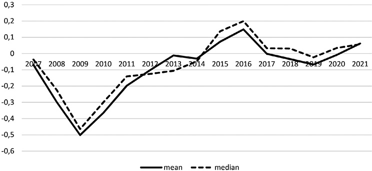
Figure 1. Mean and median of the fiscal balance of the local government sector in GDP (%) in the analysed 27 OECD countries in years 2007–2021
Source: own study.
The results of the regressions for the single factor models indicate that there are some fiscal, financial and economic variables, which show statistically significant impact on the ‘FB’ as single predictors in the models for which the p-value and the F test/Wald test do not exceed 1%. Thus, the deterioration of the ‘FB’ resulted from an increase of the change in the debt ratio (‘dDebt’), the fiscal decentralisation on the expenditure side (‘FDexp’), the investment activity (‘Inv’), the change in the unemployment rate (‘dUnemp’), or the inflation (‘Infl’). An increase of the GDP growth (‘GDPgr’), the Human Development Index (HDI) or the trade openness (Open), in contrast, positively affected the growth of ‘FB’ according to the single factor models (Table 2).
As far as the panel models for certain sets of statistically significant factors determining ‘FB’ in the OECD countries, there were estimated eight regressions (Table 3). According to the Models: 1a, 1b, 2a, 2b, 4a, 4b, between 2007 and 2021 an increase of the expenditure side of the fiscal decentralisation (‘FDexp’) affected a deterioration of fiscal balance in GDP (‘FB’). Furthermore, an increase of the change in debt ratio (‘dDebt’) resulted in a deterioration of ‘FB’ (Models: 3a, 3b, 4a, 4b). The ‘FB’ was also negatively affected by a rising inflation (Models: 1a, 1b, 2a, 2b, 4a, 4b). On the other side, the higher the trade openness (‘Open’) the more favourable fiscal balance in GDP (Models: 1a, 1b, 2a, 2b). In addition, ongoing local elections contributed to weakening of ‘FB’ (Models: 1a, 1b, 3a, 3b). Thus, in the OECD countries between 2007 and 2021 there was an electoral fiscal cycle in the field of “FB” in the local government sector. Moreover, according to the ‘Model 3a’, an increase of the Human Development Index affected a better fiscal position in the field of ‘FB’. However, this relationship was not confirmed by the ‘Model 3b’ (GMM model), in which ‘HDI’ was excluded due to its statistical insignificance.
Table 2. Potential fiscal balance factors – results of single factor models and descriptive statistics for the analysed OECD countries in the period 2007–2021
| Model for variable |
Single factor models |
Descriptive statistics |
| Type |
β |
Cons |
F test/Wald test |
Within R2 |
No. |
Mean |
Sd. |
Min |
Max |
|
Dependent variable
|
|
FB
|
–
|
–
|
–
|
–
|
–
|
405
|
–0.0937
|
0.4218
|
–1.7972
|
2.4756
|
|
Explanatory variables
|
|
FDexp
|
FE
|
–0.0716***
|
1.6026***
|
[0.0001]
|
0.1140
|
405
|
23.7047
|
12.2232
|
5.6045
|
64.6816
|
|
FA
|
FE
|
0.0126
|
–0.6489
|
[0.3017]
|
0.0126
|
405
|
58.3865
|
20.6128
|
4.0876
|
96.7957
|
|
Inv
|
RE
|
–0.0147***
|
0.4911***
|
[0.0001]
|
0.0815
|
405
|
39.6941
|
11.1556
|
14.6000
|
68.6100
|
|
dDebt
|
FE
|
–0.3713***
|
–0.0625***
|
[<0.0001]
|
0.3416
|
405
|
0.0840
|
0.5717
|
–2.8001
|
2.6427
|
|
HDI
|
FE
|
8.7564
|
–7.9647
|
[0.0014]
|
0.1144
|
405
|
0.8989
|
0.0362
|
0.8170
|
0.9620
|
|
GDPgr
|
RE
|
0.0212***
|
–0.1255**
|
[<0.0001]
|
0.0538
|
405
|
1.5011
|
3.8907
|
–14.8386
|
24.3705
|
|
Open
|
FE
|
0.0085**
|
–1.0806**
|
[0.0167]
|
0.0894
|
405
|
115.9259
|
59.8397
|
45.4188
|
388.1204
|
|
Infl
|
RE
|
–0.0481***
|
–0.0025
|
[<0.0001]
|
0.0587
|
405
|
1.8965
|
1.9846
|
–4.4781
|
15.4023
|
|
Popgr
|
RE
|
–0.0746
|
–0.0651
|
[0.2626]
|
0.0104
|
405
|
0.3832
|
0.7636
|
–2.2585
|
2.8910
|
|
dUnemp
|
RE
|
–0.0727***
|
–0.0952**
|
[0.0001]
|
0.1012
|
405
|
–0.0209
|
1.5266
|
–4.3710
|
4.3800
|
|
dIntr
|
RE
|
–0.0330**
|
–0.1015**
|
[0.0446]
|
0.0162
|
405
|
–0.2347
|
1.3254
|
–12.4433
|
8.3966
|
|
Corrupt
|
FE
|
0.8821
|
–3.7201
|
[0.3992]
|
0.0195
|
270
|
4.2205
|
0.2133
|
3.5835
|
4.5218
|
|
Elect
|
RE
|
–0.1862***
|
–0.0667
|
[<0.0001]
|
0.0402
|
315
|
–
|
–
|
–
|
–
|
Note: ***, ** and * denotes statistical significance at 1%, 5% and 10% levels respectively, for the models, in which clustered standard errors applied; p-value in brackets […]
Source: own study
Table 3. Estimation results for FE and GMM models characterizing factors affecting fiscal balance in GDP (FB, %) in the OECD countries in the period 2007–2021
| Variable |
Model 1a |
Model 1b |
Model 2a |
Model 2b |
Model 3a |
Model 3b |
Model 4a |
Model 4b |
| FE |
GMM |
FE |
GMM |
FE |
GMM |
FE |
GMM |
|
FBt–1
|
–
|
0.4419***
(0.0981)
|
–
|
0.4671***
(0.0857)
|
–
|
0.3041***
(0.0878)
|
–
|
0.3164***
(0.0627)
|
|
FDexp
|
–0.0522***
(0.0147)
|
–0.0917**
(0.0433)
|
–0.0534***
(0.0122)
|
–0.0990**
(0.0409)
|
–
|
–
|
–0.0562***
(0.0146)
|
–0.1077***
(0.0326)
|
|
Inv
|
–
|
–
|
–
|
–
|
–0.0071*
(0.0041)
|
–0.0105***
(0.0056)
|
–
|
–
|
|
dDebt
|
–
|
–
|
–
|
–
|
–0.3417***
(0.0707)
|
–0.2299***
(0.0681)
|
–0.3472***
(0.0543)
|
–0.2376***
(0.0403)
|
|
HDI
|
–
|
–
|
–
|
–
|
5.2705**
(2.4262)
|
–
|
–
|
–
|
|
Open
|
0.0062*
(0.0031)
|
0.0091**
(0.0036)
|
0.0061**
(0.0029)
|
0.0093**
(0.0037)
|
–
|
–
|
–
|
–
|
|
Inf
|
–0.0380***
(0.0062)
|
–0.0257**
(0.0108)
|
–0.0308***
(0.0061)
|
–0.0199*
(0.0109)
|
–
|
–
|
–0.0234***
(0.0077)
|
–0.0191***
(0.0061)
|
|
Elect
|
–0.1930***
(0.0366)
|
–0.1618***
(0.0345)
|
–
|
–
|
–0.1669***
(0.0288)
|
–0.1430***
(0.0394)
|
–
|
–
|
|
Cons
|
0.5112
(0.5066)
|
0.9506
(1.1484)
|
0.5280
(0.4101)
|
1.0323
(0.9919)
|
–4.4586*
(2.1448)
|
0.4154***
(0.2207)
|
1.3112***
(0.3385)
|
2.3251***
(0.8253)
|
|
Obs
|
315
|
273
|
405
|
351
|
315
|
273
|
405
|
351
|
|
Within R2
|
0.2439
|
–
|
0.1872
|
–
|
0.4604
|
|
0.4382
|
–
|
|
F test/Wald test
|
[<0.0001]
|
[<0.0001]
|
[<0.0001]
|
[<0.0001]
|
[<0.0001]
|
[<0.0001]
|
[<0.0001]
|
[<0.0001]
|
|
AR(1)
|
–
|
[0.0253]
|
–
|
[0.0183]
|
–
|
[0.0173]
|
–
|
[0.0079]
|
|
AR(2)
|
–
|
[0.8783]
|
–
|
[0.6043]
|
–
|
[0.4137]
|
–
|
[0.5595]
|
|
Sargan
|
–
|
[0.2322]
|
–
|
[0.3063]
|
–
|
[0.1685]
|
–
|
[0.4120]
|
|
Instruments No
|
–
|
18
|
–
|
17
|
–
|
17
|
–
|
17
|
Note: ***, ** and * denotes statistical significance at 1%, 5% and 10% levels respectively; cluster standard errors for FE and WC-robust standard errors for GMM in parentheses (…); p-value in brackets […]; Sargan test reported for GMM with standard errors
Source: own study.
Table 4. Estimation results for MM-QR models characterizing factors affecting fiscal balance in GDP (FB, %) in the OECD countries in the period 2007–2021
| Variable/Test |
Quantiles |
Variable/Test |
Quantiles |
| 25th |
50th |
75th |
25th |
50th |
75th |
|
Model 1q
|
Model 3q
|
|
FDexp
|
–0.0586***
(0.0222)
|
–0.0519***
(0.0169)
|
–0.0451**
(0.0221)
|
Inv
|
–0.0112***
(0.0043)
|
–0.0069**
(0.0032)
|
–0.0034
(0.0043)
|
|
Open
|
0.0071***
(0.0018)
|
0.0062***
(0.0014)
|
0.0052***
(0.0018)
|
dDebt
|
–0.3540***
(0.0499)
|
–0.3411***
(0.0369)
|
–0.3305***
(0.0494)
|
|
Inf
|
–0.0351***
(0.0132)
|
–0.0381***
(0.0100)
|
–0.0412***
(0.0131)
|
HDI
|
5.5594***
(1.7290)
|
5.2563***
(1.2766)
|
5.0067***
(1.7106)
|
|
Elect
|
–0.2032***
(0.0613)
|
–0.1926***
(0.0467)
|
–0.1818***
(0.0611)
|
Elect
|
–0.1430***
(0.0519)
|
–0.1681***
(0.0384)
|
–0.1888***
(0.0513)
|
|
Wald test
|
[<0.01]
|
[<0.01]
|
[<0.01]
|
Wald test
|
[<0.01]
|
[<0.01]
|
[<0.01]
|
|
Model 2q
|
Model 4q
|
|
FDexp
|
–0.0599***
(0.0206)
|
–0.0525***
(0.0145)
|
–0.0473***
(0.0181)
|
FDexp
|
–0.0590***
(0.0152)
|
–0.0561***
(0.0115)
|
–0.0535***
(0.0150)
|
|
Open
|
0.0072***
(0.0018)
|
0.0059***
(0.0013)
|
0.0050***
(0.0016)
|
dDebt
|
–0.3672***
(0.0378)
|
–0.3470***
(0.0285)
|
–0.3282***
(0.0371)
|
|
Inf
|
–0.0301**
(0.0144)
|
–0.0309***
(0.0101)
|
–0.0315**
(0.0126)
|
Inf
|
–0.0273**
(0.0125)
|
–0.0234** (0.0095)
|
–0.0198
(0.0123)
|
|
Wald test
|
[<0.01]
|
[<0.01]
|
[<0.01]
|
Wald test
|
[<0.01]
|
[<0.01]
|
[<0.01]
|
Note: ***, ** and * denotes statistical significance at 1%, 5% and 10% levels respectively; standard errors in parentheses (…); p-value in brackets […]
Source: own study.
Simultaneously, ‘Model 3a’ and ‘Model 3b’ indicate that a deterioration of ‘FB’ was driven by the growth of the investment activity in the local government sector. GMM models also showed a direct relationship between ‘FB’ and ‘FBt-1’. Thus, the better fiscal balance in the previous budgetary year, the more favourable this category in the current year (Table 3). On the other side, there was a pressure for the chronic deficit, e.g., due to the decline in GDP growth, which affected fiscal capacity or the need for the growth of the social spending programmes. In addition, in the estimated models the variable representing the corruption, i.e., ‘Corrupt’ was not included due to the coefficient of ‘Corrupt’ was not statistically significant. The coefficient of the corruption indicator was also not statistically significant in the single factor model. However, it revealed the positive coefficient sign in a single factor model (Table 2). It is worth noting that ‘Model 3a’ has the highest level of ‘Within R2’ of the estimated FE models, i.e., 46% of the variation in the fiscal balance in GDP within the countries is captured by this model (Table 3).
The MM-QR models also confirmed that an increase of the fiscal decentralisation on the expenditure side (‘FDexp’), the investment activity (‘Inv’), a change in the debt ratio (‘dDebt’), and an inflation (‘Inf’) contributed to a deterioration of ‘FB’ (Table 4). However, according to the ‘Model 3q’ and ‘Model 6q’ (Table 5) the inverse relationship between ‘Inv’ and ‘FB’ is not statistically significant for the 75th quantile. Thus, according to the ‘Model 3q’ and ‘Model 6q’, a typical country would experience a greater deterioration of ‘FB’ resulting from the intense investment activity if it is ranked at the lower quantile in comparison to the situation if it is ranked at the higher quantile of the distribution of ‘FB’ (Table 4, Table 5, Figure 2). Similarly, the ‘Model 4q’ shows that the impact of the inflation was not statistically significant for the 75th quantile. In addition, the MM-QR models confirmed that local elections contributed to the worsening of ‘FB’ (Table 4, Table 5, Figure 2). On the other side, an increase of the trade openness (‘Open’), and the Human Development Index (‘HDI’) affected an increase of ‘FB’. However, the impact of these two factors were higher if the country was ranked at the lower quantile in comparison to the situation if it was ranked at the higher quantile of the distribution of ‘FB’ (Table 4). Although in the FE models, as aforementioned, the ‘Corrupt’ was not included and due to this was not statistically significant, the MM-QR approach shows this is significant for 25th and 50th quantiles (Table 5). According to the ‘Model 6q’, a typical country would experience an improvement of ‘FB’ resulting from an increase of the ‘Corrupt’ (higher scores of CPI, i.e. ‘Corrupt’ indicate less corruption) if it is ranked at the 25th or 50th quantile in comparison to the situation if it is ranked at the 75th quantile of the distribution of ‘FB’ (Table 5).
Table 5. Estimation results for MM-QR and FE models characterizing factors affecting fiscal balance in GDP (FB, %) in the OECD countries in the period 2012–2021
| Variable/Test |
Quantiles |
FE |
Variable/Test |
Quantiles |
FE |
| 25th |
50th |
75th |
25th |
50th |
75th |
| Model 5q |
Model 5fe |
Model 6q |
Model 6fe |
|
Inv
|
–0.0157***
(0.0048)
|
–0.0128***
(0.0045)
|
–0.0089
(0.0070)
|
–0.0123*
(0.0067)
|
Inv
|
–0.0158***
(0.0055)
|
–0.0129***
(0.0047)
|
–0.0089
(0.0069)
|
–0.0124*
(0.0066)
|
|
dDebt
|
–0.2684***
(0.0505)
|
–0.2832***
(0.0468)
|
–0.3030***
(0.0736)
|
–0.2856***
(0.0666)
|
dDebt
|
–0.2685***
(0.0557)
|
–0.2821***
(0.0474)
|
–0.3011***
(0.0693)
|
–0.2848***
(0.0665)
|
|
HDI
|
0.2798
(2.1868)
|
1.2642
(2.0310)
|
2.5799
(3.1907)
|
1.4267
(2.1003)
|
HDI
|
–
|
–
|
–
|
–
|
|
Elect
|
–0.0952**
(0.0466)
|
–0.1218***
(0.0433)
|
–0.1574***
(0.0680)
|
–0.1262***
(0.0311)
|
Elect
|
–0.0930*
(0.0522)
|
–0.1194***
(0.0445)
|
–0.1561**
(0.0649)
|
–0.1247***
(0.0314)
|
|
Corrupt
|
1.2494**
(0.6208)
|
1.2522**
(0.5757)
|
1.2558
(0.9064)
|
1.2526
(0.9563)
|
Corrupt
|
1.2490*
(0.6909)
|
1.2803**
(0.5873)
|
1.3237
(0.8582)
|
1.2865
(0.9153)
|
|
Cons
|
–
|
–
|
–
|
–6.0398
(3.9319)
|
cons
|
–
|
–
|
–
|
–4.8948
(4.0144)
|
|
Wald test
|
[<0.01]
|
[<0.01]
|
[<0.01]
|
[<0.01]
|
Wald test
|
[<0.01]
|
[<0.01]
|
[<0.01]
|
[<0.01]
|
|
Obs
|
210
|
210
|
Obs
|
210
|
210
|
Note: ***, ** and * denotes statistical significance at 1%, 5% and 10% levels respectively; standard errors for MM-QR and cluster standard errors for FE in parentheses (…); p-value in brackets […]
Source: own study.
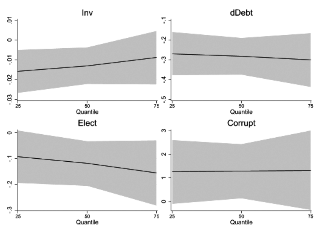
Figure 2. Coefficients of the fiscal balance factors (solid black lines) at the background of 95% confidence intervals (grey areas) in the Model 6q (MM-QR) across different quantiles
Source: own study.
It is worth adding that the explanatory variables in the FE, GMM and MM-QR models show a joint statistical significance (F test or Wald test) (Table 3, Table 4, Table 6). Moreover, in the case of GMM models the diagnostic tests are correct, i.e., the Sargan test shows that the instruments in all estimations are valid along with the tests for serial correlation finding no significant evidence of serial correlation in the first-differenced errors at order 2. In turn, the levels of VIF indicate that a multicollinearity is not a cause for concern, while the Hausman test results confirm that the use of the models with fixed effects, i.e., Models: 1q, 2q, 3q, 4q, was appropriate (Table 6). The Pesaran CD test shows that the variables have the presence of cross-sectional dependence, whereas the CIPS test indicates that some variables are borderline between I(0) and I(1) (Table 6).
Table 6. Diagnostic tests and the statistics concerning MM-QR models
|
Details
|
Model 1q
|
Model 2q
|
Model 3q
|
Model 4q
|
|
CD
test
|
CIPS without trend
|
CIPS with trend
|
CD
test
|
CIPS without trend
|
CIPS with trend
|
CD
test
|
CIPS without trend
|
CIPS with trend
|
CD
test
|
CIPS without trend
|
CIPS with trend
|
|
FB
|
[<0.01]
|
[<0.01]
|
[<0.01]
|
[<0.01]
|
[<0.01]
|
[<0.01]
|
[<0.01]
|
[<0.01]
|
[<0.01]
|
[<0.01]
|
[<0.01]
|
[<0.01]
|
|
FDexp
|
[<0.01]
|
[0.62]
|
[0.22]
|
[<0.01]
|
[0.50]
|
[0.44]
|
–
|
–
|
–
|
[<0.01]
|
[<0.50]
|
[<0.44]
|
|
Inv
|
–
|
–
|
–
|
–
|
–
|
–
|
[<0.01]
|
[0.19]
|
[0.04]
|
–
|
–
|
–
|
|
dDebt
|
–
|
–
|
–
|
–
|
–
|
–
|
[<0.01]
|
[<0.01]
|
[0.04]
|
[<0.01]
|
[<0.01]
|
[0.02]
|
|
HDI
|
–
|
–
|
–
|
–
|
–
|
–
|
[<0.01]
|
[<0.01]
|
[0.16]
|
–
|
–
|
–
|
|
Open
|
[<0.01]
|
[0.58]
|
[0.96]
|
[<0.01]
|
[0.63]
|
[0.99]
|
–
|
–
|
–
|
–
|
–
|
–
|
|
Inf
|
[<0.01]
|
[0.01]
|
[0.07]
|
[<0.01]
|
[0.01]
|
[0.23]
|
–
|
–
|
–
|
[<0.01]
|
[0.01]
|
[<0.23]
|
|
Elect
|
[<0.01]
|
[<0.01]
|
[<0.01]
|
–
|
–
|
–
|
[<0.01]
|
[<0.01]
|
[<0.01]
|
–
|
–
|
–
|
|
Max VIF
|
1.12
|
1.09
|
1.08
|
1.04
|
|
Mean VIF
|
1.07
|
1.06
|
1.04
|
1.03
|
|
Hausman test
|
[<0.01]
|
[<0.01]
|
[<0.01]
|
[<0.01]
|
|
Obs
|
315
|
405
|
315
|
405
|
Note: p-value in brackets […]
Source: own study.
Table 7. Results of the Mann–Whitney U test, Kruskal–Wallis test, Dunn test for only significant statistics at the p-value 0.1 for the ‘FB’ for the CEE and the non-CEE countries in the period 2007–2021 against the background of mean and median of ‘FB’ and ‘GDP growth’
| Test |
Year |
| 2009 |
2015 |
2016 |
2020 |
|
Mann–Whitney U
|
[0.0949]
|
[0.0662]
|
[0.0217]
|
[0.1795]
|
|
Kruskal–Wallis
|
[0.0893]
|
[0.0631]
|
[0.0224]
|
[0.1674]
|
|
Dunn
|
[0.0446]
|
[0.0316]
|
[0.0224]
|
[0.0837]
|
|
Mean and median of ‘FB’
|
|
Mean for the CEE countries
|
–0.7283
|
0.2423
|
0.2422
|
0.1195
|
|
Mean for the non-CEE countries
|
–0.4056
|
0.0014
|
0.0459
|
–0.0624
|
|
Median for the CEE countries
|
–0.5184
|
0.2560
|
0.2773
|
0.1250
|
|
Median for the non-CEE countries
|
–0.3251
|
–0.0046
|
0.0655
|
–0.0386
|
|
Mean and median of ‘GDP growth’, %
|
|
Mean for the CEE countries
|
–8.1443
|
3.5774
|
2.6088
|
–2.8178
|
|
Mean for the non-CEE countries
|
–4.1720
|
3.1026
|
2.2295
|
–4.8439
|
|
Median for the CEE countries
|
–7.0732
|
3.7963
|
2.5281
|
–2.7888
|
|
Median for the non-CEE countries
|
–3.7646
|
1.9592
|
2.0687
|
–5.2330
|
Note: p-value in brackets […]; the results of the tests were presented if the p-value of at least one test was below 0.1 for each year between 2007–2021
Source: own study.
Furthermore, the results of the Mann-Whitney U test, Kruskal–Wallis test, Dunn test showed that there were differences in the distribution of the fiscal balance of local government sector in GDP, % (‘FB’) between the CEE and the non-CEE countries in some years between 2007 and 2021 (Table 7). In the aftermath of the global financial crisis, i.e., in 2009 there were differences in the distribution of ‘FB’. In 2009 the median of ‘FB’ of the CEE countries were lower in comparison to the non-CEE countries. In the group of the CEE countries there were also less favourable levels of the median and the mean of GDP growth in 2009. Moreover, in the years: 2015 and 2016 there were also differences in the distribution of ‘FB’ between the analysed groups of countries (Table 7). In these cases, the medians of ‘FB’ were higher, along with the higher median of GDP growth. In 2020, i.e., in the year of the Covid outbreak, only the Dunn test showed statistically significant differences (at the p-value 0.1) in the levels of ‘FB’ between the CEE and the non-CEE countries, along with the differences in the median and the mean of GDP growth.
Conclusion
The level of fiscal balance in the local government sector is a key issue determining its fiscal sustainability and the exposure to fiscal distress. The fiscal balance may also affect financial circumstances of the business sector, especially an access to external sources of funding. Therefore, it is crucial to examine its potential determinants to avoid chronic deficit contributing to the deterioration of fiscal balance in subsequent periods.
The conducted research shows that the level of fiscal balance of the local government sector in GDP (‘FB’) is determined by the fiscal, economic, political and institutional factors. The empirical models revealed that an increase of the fiscal decentralisation on the expenditure side and an intense investment activity in the local government sector affect a deterioration of ‘FB’. Simultaneously, a typical country would experience a greater worsening of ‘FB’ because of the intense investment activity at the local level if it is ranked at the lower quantile in comparison to the situation if it is ranked at the higher quantile of the distribution of ‘FB’. Thus, the public authorities should improve ‘FB’ in the eve of the higher capital spendings to increase the financial resilience. In addition, an increase of the changes in the indebtedness of local government sector contributes to worsening of ‘FB’. Thus, these fiscal ratios are key fiscal balance factors and could be applied as significant explanatory variables in the single factor models. Thus, both the hypothesis 1 (H1) and the hypothesis 2 (H2) were positively verified. Similarly to the findings of Crivelli (2012), the research study showed that there is little that fiscal autonomy can do to induce fiscal discipline at the local government level from the international perspective. On the other side, an increase of the trade openness contributes to the improvement of ‘FB’, which is in line with the aforementioned study of Crivelli (2012). Hence, the hypothesis 3 (H3) was positively verified. The positive impact of an increase in the trade openness and also the Human Development Index on ‘FB’, is higher if a country is at the lower quantile compared to when it is at the upper quantile of the distribution of the fiscal balance in GDP. Simultaneously, to avoid negative aspects of the trade openness, indicated by Combes and Saadi-Sedik (2006) sound budget institutions should be designed and implemented, especially to insulate public spending from political pressures. Sound fiscal institutions could also alleviate the negative impact of the corruption on the ‘FB’. The outcomes of the panel quantile regression with fixed effects confirm the hypothesis 5 (H5) stating that there is a direct relationship between the Corruption Perception Index and ‘FB’. However, this relationship is statistically significant if the country is ranked at the 25th and 50th quantiles of ‘FB’, rather than if it is ranked at the 75th quantile of ‘FB’. Thus, the current fiscal position determines the significance of the impact of the corruption on the fiscal balance. Moreover, counteracting corruption becomes particularly important in countries characterized by weak ‘FB’ in order to enhance fiscal sustainability. The scholars also indicate that the corruption contributes to the growth of tax evasion, a shadow economy, or inefficiency of the spending policy, which impact the fiscal balance. Furthermore, the estimated regressions showed that local elections affect the deterioration of the fiscal balance of the local government sector in GDP. Thus, the electoral fiscal cycle was confirmed, which was also proved by Veiga and Veiga (2014), Działo et al. (2019), Köppl Turyna et al. (2016), who explored these relationships from a national perspective. The positive verification of hypothesis 6 (H6) means that upcoming local elections contributes to the loosening of fiscal policy in the local government sector, and negatively affects the fiscal sustainability. This relationship can be particularly dangerous in the period of rising inflation. The findings displayed that there is an inverse relationship between an inflation and ‘FB’. Hence, the hypothesis 4 (H4) was positively verified. Moreover, the public authorities should pay particular attention to reducing unemployment to increase tax capacity and decrease the social spendings. In addition, changes in the interest rates affect ‘FB’, e.g., determining current expenditures on debt servicing. Thus, the authorities should be aware that larger increases in the debt ratio, worsening the ‘FB’, additionally expose to the interest rate risk. To sum up, maintaining a sound fiscal balance improves financial resilience of the local government.
Simultaneously, the findings show that in some years of the analysed period there were differences in the distribution of the ‘FB’ between the CEE and the on-CEE countries, which were accompanied by differences in the level of the median and the mean of GDP growth. In particular, in 2009, in the CEE countries ‘FB’ was strongly affected by the global financial crisis, whereas in 2015 and 2016 these countries achieved better fiscal positions in the field of ‘FB’. Therefore, it is worth examining additional institutional factors, which differentiate these countries in the field of fiscal balance, and could affect the fiscal sustainability or the fiscal distress.
Paweł Galiński – Ph.D., University of Gdańsk, Faculty of Management, Department of Banking and Finance, pawel.galinski@ug.edu.pl, https://orcid.org/0000-0002-9407-4515
References
Aidt T.S. (2009), Corruption, institutions, and economic development, “Oxford Review of Economic Policy”, 25(2): 271–291. https://doi.org/10.1093/oxrep/grp012
Apergis N., Ben Ali, M.S. (2020), Corruption, Rentier States and Economic Growth Where Do the GCC Countries Stand?, [in:] H. Miniaoui (ed.), Economic Development in the Gulf Cooperation Council Countries. Gulf Studies, Vol. 1. Springer, Singapore. https://doi.org/10.1007/978-981-15-6058-3_6
Baltagi B.H. (2021), Econometric Analysis of Panel Data, Sixth Edition, Springer, Cham.
Barreto H., Howland, F. (2006), Introductory Econometrics: Using Monte Carlo Simulation with Microsoft Excel, Cambridge University Press, New York.
Benito B., Guillamón M.-D., Ríos A.-M. (2021), Political Budget Cycles in Public Revenues: Evidence From Fines, “SAGE Open”, 11(4). https://doi.org/10.1177/21582440211059169
Bernheim B.D. (1989), A Neoclassical Perspective on Budget Deficits, “Journal of Economic Perspectives”, 3(2): 55–72. https://doi.org/10.1257/jep.3.2.55
Beyaert A., García-Solanes J., Lopez-Gomez L. (2023), Corruption, quality of institutions and growth, “Applied Economic Analysis”, 31(91): 55–72. https://doi.org/10.1108/AEA-11-2021-0297
Bonfatti A., Forni L. (2019), Fiscal rules to tame the political budget cycle: Evidence from Italian municipalities, “European Journal of Political Economy”, 60: 1–20. https://doi.org/10.1016/j.ejpoleco.2019.06.001
Brown-Collier E.K., Collier B.E. (1995), What Keynes Really Said about Deficit Spending, “Journal of Post Keynesian Economics”, 17(3): 341–355. https://doi.org/10.1080/01603477.1995.11490034
Bukowska G., Siwińska-Gorzelak J. (2016), Can Fiscal Decentralisation Curb Fiscal Imbalances?, University of Warsaw, Faculty of Economic Science, “Working Papers”, 35(226).
Cifuentes-Faura J., Simionescu M., Gavurova B. (2022), Determinants of local government deficit: evidence from Spanish municipalities, “Heliyon”, 8(12): 1–11. https://doi.org/10.1016/j.heliyon.2022.e12393
Combes J.-L., Saadi-Sedik T. (2006), How Does Trade Openness Influence Budget Deficits in Developing Countries?, “IMF Working Paper”, 3.
Crivelli E. (2012), Local Governments’ Fiscal Balance, Privatization, and Banking Sector Reform in Transition Countries, “IMF Working Paper”, 146.
Das P. (2019), Econometrics in Theory and Practice. Analysis of Cross Section, Time Series and Panel Data with Stata 15.1, Singapore, Springer.
Dreher A., Schneider F. (2010), Corruption and the shadow economy: an empirical analysis, “Public Choice”, 144: 215–238. https://doi.org/10.1007/s11127-009-9513-0
Drissen G.A. (2022), Deficits, Debt, and the Economy: An Introduction, Deficits. Updated December 20, “Congressional Research Service”, R44383.
Działo J., Guziejewska B., Majdzińska A., Żółtaszek A. (2019), Determinants of Local Government Deficit and Debt: Evidence from Polish Municipalities, “Lex Localis – Journal of Local Self-Government”, 17(4): 1033–1056. https://doi.org/10.4335/17.4.1033-1056(2019)
Filipiak B.Z., Wyszkowska D. (2022), Stabilność fiskalna w krajach UE, “Wiadomości Statystyczne. The Polish Statistician”, 67(8): 17–40. https://doi.org/10.5604/01.3001.0015.9703
Fischer S., Easterly W. (1990), The Economics of the Government Budget Constraint, “The World Bank Research Observer”, 5(2): 127–142. https://doi.org/10.1093/wbro/5.2.127
Galiński P. (2021), Zagrożenie fiskalne jednostek samorządu terytorialnego. Uwarunkowania, pomiar, ograniczanie, Wydawnictwo Uniwersytetu Gdańskiego, Gdańsk–Sopot.
Galiński P. (2022), Importance of the Size of Local Government in Avoiding the Fiscal Distress – Empirical Evidence on Communes in Poland, “Annales Universitatis Mariae Curie-Skłodowska, sectio H – Oeconomia”, 56(5): 101–113. https://doi.org/10.17951/h.2022.56.5.101-113
Galiński, P. (2023a), Key Debt Drivers of Local Governments: Empirical Evidence on Municipalities in Poland, Lex Localis - Journal of Local Self-Government, 21(3): 591–618. https://doi.org/10.4335/21.3.591-618(2023)
Galinski P. (2023b), Determinants of debt for local governments in Europe – panel data research, “Forum Scientiae Oeconomia”, 11(2): 69–86. https://doi.org/10.23762/FSO_VOL11_NO2_3
Gnimassoun B., Do Santos I. (2021), Robust structural determinants of public deficits in developing countries, “Applied Economics”, 53(9): 1052–1076. https://doi.org/10.1080/00036846.2020.1824063
Gruszczyński M. (2020), Financial Microeconometrics. A Research Methodology in Corporate Finance and Accounting, Springer, Cham.
Hemming R., Mahfouz S., Schimmelpfennig A. (2002), Fiscal Policy and Economic Activity During Recessions in Advanced Economies, “IMF Working Paper”, 87.
Hill R.C., Griffiths W.E., Lim, G.C. (2018), Principles of Econometrics, Fifth Edition, John Wiley & Sons, Hoboken.
Jacquemet N., L’Haridon O. (2018), Experimental Economics. Methods and Applications, Cambridge University Press, Cambridge.
Kacapyr E. (2022), Essential Econometric Techniques A Guide to Concepts and Applications, Third Edition, Routledge, New York.
Kłysik-Uryszek A., Uryszek T. (2022), Public Debt Sustainability and the COVID Pandemic: The Case of Poland, “Central European Economic Journal”, 9(56): 68–75. https://doi.org/10.2478/ceej-2022-0005
Koengkan M., Fuinhas J.A., Tavares A.I.P, Silva N.M.B.G. (2023), Obesity Epidemic and the Environment Latin America and the Caribbean Region, Elsevier, London.
Köppl Turyna M., Kula G., Balmas A., Waclawska K. (2016), The effects of fiscal decentralisation on the strength of political budget cycles in local expenditure, “Local Government Studies”, 42(5): 785–820. https://doi.org/10.1080/03003930.2016.1181620
Lami E. (2023), Political Budget Cycles in the Context of a Transition Economy: The Case of Albania, “Comparative Economic Studies”, 65: 221–262. https://doi.org/10.1057/s41294-022-00191-6
Lis E.M, Nickel C. (2010), The impact of extreme weather events on budget balances, “International Tax and Public Finance”, 17(4): 378–399. http://hdl.handle.net/10.1007/s10797-010-9144-x
Machado J.A.F., Santos Silva J.M.C. (2019), Quantiles via Moments, “Journal of Econometrics”, 213(1): 145–173. https://doi.org/10.1016/j.jeconom.2019.04.009
Mawejje J., Odhiambo N.M. (2022), Macroeconomic determinants of fiscal policy in East Africa: a panel causality analysis, “Journal of Economics, Finance and Administrative Science”, 27(53): 105–123. https://doi.org/10.1108/JEFAS-07-2021-0124
Muluk M.R.K., Wahyudi L.E. (2022), Key Success in Fostering Human Development Index at the Local Level, “Otoritas: Jurnal Ilmu Pemerintahan”, 12(2): 128–141. https://doi.org/10.26618/ojip.v12i2.7665
National Research Council (NTC) and National Academy of Public Administration (NAPA), (2010), Choosing the Nation’s Fiscal Future, The National Academies Press, Washington, DC.
OECD (2021), Government at a Glance 2021, OECD Publishing, Paris. https://doi.org/10.1787/1c258f55-en.
Organisation for Economic Co-operation and Development (OECD), https://stats.oecd.org/ (accessed: 16.05.2023)
Organisation for Economic Co-operation and Development (OECD), https://www.oecd.org/tax/federalism/fiscal-decentralisation-database/ (accessed: 16.05.2023)
Pinardon-Touati N. (2022), The Crowding Out Effect of Local Government Debt: Micro and Macro-Estimates, “Working Paper”, HEC Paris.
Postiglione P. (2022), Spatial Panel Regression Models in R, [in:] P. Postiglione, R. Benedetti, F. Piersimoni (eds.), Spatial Econometric Methods in Agricultural Economics Using R, Taylor & Francis Group, Boca Raton.
Rangarajan C., Srivastava D.K. (2005), Fiscal Deficits and Government Debt: Implications for Growth and Stabilisation, “Economic and Political Weekly”, 40(27): 2919–2934.
Shah A. (2005), Fiscal decentralization and fiscal performance, “World Bank Policy Research Working Papers”, 3786.
Simionescu M., Cifuentes-Faura J. (2023), Public Debt in the Spanish Municipalities: Drivers and Policy Proposals, “Evaluation Review”, 0(0): 1–32. https://doi.org/10.1177/0193841X231193465
Sinervo L.-M. (2020), Financial Sustainability of Local Governments in the Eyes of Finnish Local Politicians, “Sustainability”, 12(10207): 1–16. https://doi.org/10.3390/su122310207
Sonmez Ozekicioglu S., Yaraşır Tülümce S. (2020). The Impacts of Corruption on Budget Balance and Public Debt in Turkey: an Empirical Analysis, “Journal of Management and Economics Research”, 18(3): 46–60. https://doi.org/10.11611/yead.775529
Sow M., Razafimahefa I. (2017), Fiscal Decentralization and Fiscal Policy Performance, “IMF Working Paper”, 64.
Tanzi V., Davoodi H. (2001), Corruption, growth, and public finances, [in:] A.K. Jain (ed.), The Political Economy of Corruption, Routledge, London–New York.
Teixeira A.A.C., Guimarães L. (2015), Corruption and FDI: Does the Use of Distinct Proxies for Corruption Matter?, “Journal of African Business”, 16(1–2): 159–179. https://doi.org/10.1080/15228916.2015.1027881
Transparency International (2022), Corruption Perceptions Index 2021, Berlin.
Transparency International (TI), https://www.transparency.org/en/cpi/ (accessed: 18.05.2023).
Tujula M., Wolswijk G. (2004), What Determines Fiscal Balances? An Empirical Investigation in Determinants of Changes in OECD Budget Balances, “European Central Bank Working Paper Series”, 422.
UN-HABITAT (2015), The Challenge of Local Government Financing in Developing Countries, United Nations Human Settlements Programme, Nairobi.
United Nations Development Programme (UNDP) (2011), Towards human resilience: sustaining MDG progress in an age of economic uncertainty, UNDP, Bureau for Development Policy, New York.
Uryszek T. (2018). Fiscal Sustainability of Local Governments in the Visegrad Group Countries, “Entrepreneurial Business and Economics Review”, 6(3): 59–71. https://doi.org/10.15678/EBER.2018.060304
Uryszek T. (2020). Stabilizacja i optymalizacja długu publicznego a zrównoważenie sektora finansów publicznych: Polska na tle Unii Europejskiej, Wydawnictwo Uniwersytetu Łódzkiego, Łódź.
Veiga L.G., Veiga F.J. (2014), Determinants of Portuguese local governments’ indebtedness, “NIPE Working Papers”, 16.
Ward R.B. (2012), Achieving Fiscal Sustainability for State and Local Governments, [in:] R.D. Ebel, J.E. Petersen (eds), The Oxford Handbook of State and Local Government Finance, Oxford University Press, Oxford. https://doi.org/10.1093/oxfordhb/9780199765362.013.0033
World Bank, https://data.worldbank.org/ (accessed: 16.05.2023).
Wójtowicz K.A., Hodžić S. (2022), Financial Resilience in the Face of Turbulent Times: Evidence from Poland and Croatian Cities. “Sustainability”, 14. https://doi.org/10.3390su141710632
Yahaya B., Nkwatoh L.S, Jajere B.A. (2021), Impact of Climate Change on Budget Balance: Implications for Fiscal Policy in the ECOWAS Region, “International Journal of Economics and Finance”, 13(8): 25–30. https://doi.org/10.5539/ijef.v13n8p25
Ziolo M. (2015), Diagnosing fiscal distress: Regional evidence from Polish municipalities, “Romanian Journal of Fiscal Policy”, 6(2), 14–33.
Streszczenie
Czynniki równowagi fiskalnej samorządu terytorialnego: badanie danych panelowych dotyczące krajów OECD
Równowaga fiskalna postrzegana jest jako podstawowy miernik stabilności fiskalnej w samorządzie terytorialnym. Wpływa ona na reakcję budżetu na wypadek potencjalnej recesji, determinując zagrożenie fiskalne i odporność finansową. Stąd ekonomiści prowadzą badania w celu identyfikacji czynników oddziałujących na równowagę fiskalną na szczeblu lokalnym. Dlatego celem tego artykuły jest zbadanie czynników o charakterze fiskalnym, społeczno-ekonomicznym, politycznym i instytucjonalnym, które wpływają na poziom salda budżetowego w relacji do Produktu Krajowego Brutto (PKB) na podstawie krajów OECD w latach 2007–2021. W badaniu zastosowano modele panelowe z efektami stałymi oraz z efektami losowymi, dynamiczne modele panelowe (GMM) oraz kwantylową regresję panelową z efektami stałymi. W rezultacie potwierdzono, że na poziom salda budżetowego samorządu terytorialnego w relacji do PKB oddziałuje strona wydatkowa decentralizacji fiskalnej, aktywność inwestycyjna, zmiany wskaźnika zadłużenia, inflacja, zmiana stopy bezrobocia, Wskaźnik Rozwoju Społecznego, wymiana handlowa, wzrost PKB oraz wybory samorządowe. Ujawniono także statystyczną istotność wpływu korupcji w przypadku oszacowanych modeli kwantylowej regresji panelowej z efektami stałymi. Dodatkowo zastosowano testy statystyczne U Manna–Whitney’a, Kruskala–Wallisa oraz Dunna w celu zidentyfikowania różnic pomiędzy krajami Europy Środkowo-Wschodniej i pozostałymi państwami OECD pod względem rozkładu badanego salda budżetowego w PKB.
Słowa kluczowe: równowaga fiskalna, deficyt, stabilność fiskalna, zagrożenie fiskalne, samorząd terytorialny, wybory samorządowe, korupcja
© by the author, licensee University of Lodz – Lodz University Press, Lodz, Poland. This article is an open access article distributed under the terms and conditions of the Creative Commons Attribution license CC-BY-NC-ND 4.0 (
https://creativecommons.org/licenses/by-nc-nd/4.0/)