Introduction

The Trivers–Willard hypothesis (TWH) posits that the maximization of reproductive success in mammals is associated with modifying the sex ratio of offspring depending on maternal condition (Tri­vers and Willard 1973). As indicated by research on human populations, natural selection mechanisms decrease the male birth rate in stressful periods by reducing the number of conceptions and increasing the proportion of spontaneous abortions of male fetuses (James and Grech 2017). This implies that a long-term deterioration of living conditions (e.g., economic stress) in the human population may lead to a lower sex ratio at birth. However, research on the verification of the so-called economic stress hypothesis initiated by Catalano and Bruckner (2005) has not led to conclusive results.

That research has been based on the secondary sex ratio (SSR), which is the ratio of male to female live births (Cata­lano 2003; Catalano and Bruckner 2005; Żądzińska et al. 2007; 2011) or the human sex ratio measured as the sex ratio at birth (SRB) calculated as the proportion of male births in relation to all births (Helle et al. 2009; Wu 2021). Analysis has also included the annual number of stillbirths by sex, accounting for part of the overall number of prenatal deaths. Findings on the mortality of male and female fetuses may shed light on the mechanisms underlying the Trivers–Willard hypothesis (Catalano et al. 2005a; 2005b; Helle et al. 2009)

Research in this area is usually based on the annual number of live births by sex. The availability of birth registers and metrics describing changes in economic conditions over time in a given country have made it possible to design and conduct analyses for different periods and different human populations: for 1862–1991 and 1749–1991 in Sweden (Catalano and Bruckner 2005; Wu 2021), for 1865–2003 in Finland (Helle et al. 2009), for 1946–1999 in East and West Germany (Catalano 2003), and for 1956–2005 (Żądzińska et al. 2007) and 1995–2007 (Żądzińska et al. 2011) in Poland (with quarterly data in the latter case).

Previous research, using different measures of changes in economic conditions, has partially confirmed that an economic recession may reduce the proportion of male births. Catalano (2003), who applied time series analysis to data from East and West Germany for 1946–1999, found the SSR in East Germany in the turbulent year 1991 (1.044) to be lower than the ratio of 1.059 expected from history and from the ratio in West Germany.

Analyzing monthly data from January 1989 to December 2001, Catalano et al. (2005a) reported that the fetal death sex ratio increased in months when the unemployment rate also increased. Using demographic and economic data spanning 129 years for Sweden, Catalano and Bruckner (2005) found a positive correlation between percentage change in private consumption and the SSR in that country in the period 1862–1991.

A few subsequent studies did not report conclusive results, which indicates the need to further verify the relationship between economic stress and the sex ratio at birth (Margerison Zilko 2010). A Polish study following Catalano and Bruckner’s methodology (2005) using annual data for 1956–2005 did not reveal a correlation between consumption and the SSR (Żądzińska et al. 2007). Similarly, findings from another study using a dynamic regression model did not bear out an association between the SRB and changes in real GDP in Finland between 1865 and 2003 (Helle et al. 2009). Cata­lano and Bruckner’s analysis (2005), involving data from 1862–1991, did confirm an association between private consumption and the Swedish SSR over 129 years, while an extended research by Wu (2021), encompassing time series from almost two and a half centuries (1749–1991), was inconclusive as to the effects of economic stress on changes in the Swedish SRB.

The verification of the economic stress hypothesis requires long study periods, which may not always be possible due to the absence of data or inaccurate records of live births. In addition, in many places around the world there are no records of prenatal deaths. In the case of Poland, data on births in the interwar period (1918–1939) may be distorted as some parents may have consciously delayed birth registration or failed to register (Szukalski 2010). As was mentioned above, attempts to explain changes in the SSR in Poland by economic stress (deterioration of living conditions) over a period of 50 years (1956–2005) did not bring the expected results (Żądzińska et al. 2007). According to some Polish demographers, this may be partially attributed to the choice of indicator of living conditions in the study i.e. the private consumption of households, which may have overestimated the actual living conditions in the years of market shortages (Szukalski 2010). On the other hand, the results of another study, limited to the years following the period of political and economic transformation in Poland (1995–2007) did show a positive correlation between percentage change in private consumption and the SSR using quarterly data for Łódzkie Province (Żądzińska et al. 2011): the SSR was found to decrease four quarters after the occurrence of an economic stressor. Thus, the results may suggest that SSR fluctuations could be used as an indicator of economic stress at the population level.

Testing the Trivers–Willard hypothesis

The hypothesis posited by Trivers and Willard (TWH) initiated research on the effects of economic stress (consumption) on the number of male births in relation to that of female births. To verify the influence of the economic stress under the “incorrect“ null hypothesis (H₀) it is assumed that when consumption increases over its expected value, then the sex ratio should fall below its expected value (it is an assumption that consumption does not matter). In turn, the alternative “correct” hypothesis (H₁) assumes that lower-than-expected consumption of goods and services may cause eco­nomic stress leading to a lower SSR (it is an assumption about a positive dependence between consumption and the secondary sex ratio). Firstly, from hypothesis H₁ it follows that the observed SSR for live births should increase (as a result of a higher number of male births and/or a lower number of female births) when households consume more goods and services than they actually need. Secondly, this hypothesis suggests that the observed SSR for live births should decrease (due to a higher number of female births and/or a lower number of male births) when households consume fewer goods and services than they need.

Even though the literature does not provide a test that can directly verify this hypothesis, the authors believe that the method proposed by Catalano and Bruckner (2005) – based on an econometric model – is correct. However, the method requires time series of sufficient length and temporal resolution, proper data preparation, and appropriate time series analysis. Therefore, it is crucial to have an in-depth understanding of the procedures used to verify the posited hypothesis (see: Statistical analysis methods). In the classical theory of hypothesis verification, null and alternative hypo­theses are not treated in the same way. H₀ enjoys a certain advantage over H₁ as it can be rejected only on the basis of very substantial evidence against it, usually at a 0.05 or 0.01 alpha level.

The TWH was previously confirmed for a region in central Poland (Łódzkie Province) based on quarterly data for the years 1995–2007, following a period of political and economic transformation (Żądzińska et al. 2011). The objective of the current study is to retest the TWH, this time using semiannual time series for Łódzkie Province and a new dataset for Poland. In addition, two different measures of the human sex ratio (the SSR and SRB) are analyzed in the study. The statistical method proposed by Cata­lano and Bruckner (2005), expanded to include additional statistical analyses, is applied to retest the economic stress hypothesis in Łódzkie Province and in Poland for the years 1995–2020.

Material and methods

Research material

Research material consisted of semiannual data on the total numbers of live male births (M) and live female births (F) in the Polish population in the years 1995–2020 (52 semiannual data points) derived from balance tables of population, natural movements, and migrations. The authors had access to data for Poland and for individual regions (provinces) of the country at the NUTS-2 level (Statistics Poland). The available data were used to produce semiannual time series for the secondary sex ratio (SSR), which is the proportion of male to female births [M/F], and the sex ratio at birth (SRB), which is the proportion of male births to all births [M/(M+F)]. Fig. 1 presents SSR results for Poland and for Łódzkie Province.

In 1995–2020, the M/F ratio for Poland ranged from 1.0507 to 1.0814, with a mean of 1.0598, a standard deviation (SD) of 0.006, and a coefficient of variation (CV) of 0.58% (CV, expressed as a percentage, is the ratio of the standard deviation to the mean times 100). In the case of Łódzkie Province, the corresponding values for the M/F ratio in 1995–2020 were: 1.0198 (min), 1.1217 (max), 1.0600 (mean), 0.018 (SD), and a CV of 1.73% (Fig. 1). Diagrams plotted for the M/(M+F) ratio – despite using a different unit (%) – appeared very similar. In the years 1995–2020, SRB values ranged from 51.2% to 52.0% for Poland and from 50.5% to 52.9% for Łódzkie Province; the results for Łódzkie Province also revealed greater variation.

According to the methodology described in previous research (Catalano and Bruckner 2005; Żądzińska et al. 2011), the economic stress experienced by the population in Poland and in Łódzkie Province was expressed by means of private consumption, that is, the final consumption expenditure of households (in million units of national currency at constant 2015 prices) was based on seasonally and calendar adjusted data. In statistical analysis (ARMA models), the variable describing the economic condition of households was percentage change in private consumption [ΔC/C] (Fig. 2).

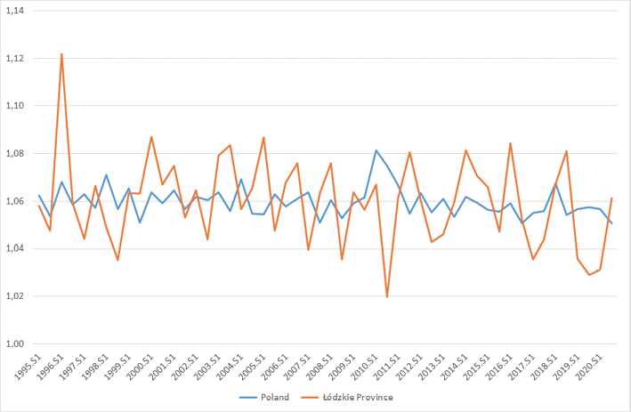
Fig. 1. M/F ratio (semiannual data) for Poland and for Łódzkie Province in 1995–2020. Authors’ calculation based on data obtained from https://demografia.stat.gov.pl/BazaDemografia/StartIntro.aspx (Statistics Poland)

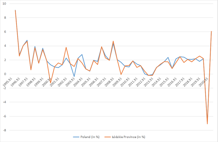
Fig. 2. Percentage change in private consumption [ΔC/C] for Poland and for Łódzkie Province in 1995–2020. Authors’ calculation based on data obtained from https://ec.europa.eu/eurostat/data/database (Economy and Finance / National accounts (ESA 2010) / Quarterly national accounts / Main GDP aggregates, Eurostat)

Percentage change in private consumption for Poland and for Łódzkie Province in the years 1995–2020 (semi­annual data) was similar. The greatest one-off drop in consumption in the study period (by approx. 7.0%) was found for the first half of 2020, at the height of the COVID-19 pandemic (Fig. 2).

Statistical analysis methods

The effects of economic stress on the SSR and SRB were analyzed using the method proposed by Catalano and Bruckner (2005) supplemented by the authors with additional calculations, marked with an asterisk in the scheme below (*).

Step 1: Testing the stationarity of the [ΔC/C], M/F, and M/(M+F) time series. The trend line slope coefficient was determined and evaluated. We used the augmented Dickey–Fuller (ADF) test and Kwiatkowski–Phillips–Schmidt–Shin (KPSS) test to evaluate stationarity of the analyzed processes. Moreover, we examined fractional integration of the time series by means of Geweke, Porter-Hudak (GPH) test (*).

Step 2: Construction of a private consumption model [ΔC/C]. Percentage change in private consumption was decomposed into statistically expected and unexpected components. The Box and Jenkins method (Box and Jenkins 1983) was applied to identify the order of the autoregressive process (AR), the moving average process (MA), and the autoregressive moving average process (ARMA) in this step and in Steps 3 and 4. The estimated values of the best-fitting Box–Jenkins model can be thought of as the expected component of the modeled series while the differences between the observed and estimated values are the unexpected component.

Step 3: Construction of the M/F model. The SSR ratio was decomposed into statistically expected and unexpected components (see: Step 2). The unexpected component of private consumption (eΔC/C – residuals) was added to the M/F model.

Step 4: Construction of the M/(M+F) model. The SRB ratio was decomposed into statistically expected and unexpected components (see: Step 2). The unexpected component of private consumption (eΔC/C – residuals) was added to the M/(M+F) model.

Step 5: Choosing the final M/F and M/(M+F) equations. The final models of the effects of economic stress on the sex ratio were selected according to the following criteria: (1) all parameters of the model were statistically different from zero, (2) the model exhibited the lowest Akaike Information Criterion (AIC), (3) the coefficient of the lagged explanatory variable (residual from the consumption model [eΔC/C(.)] was positive, and (4) the model enabled a dual solution – obtaining the same specification and (statistically different from zero) model parameters for both the SSR and SRB. This was an additional analysis measuring the stability of the association (*).

Step 6: Analysis of residuals from the model. Residuals from the final equation (stationarity, normal distribution) were evaluated and the equation was re-estimated.

Step 7: Decision making (TWH). In constructing a model explaining the SSR and SRB, the null hypothesis (H₀) is deliberately incorrect. It assumes that an improvement in economic conditions reflected in increased consumption causes a decline in the SSR and SRB (an assumption about the absence of a consumption effect), versus an alternative hypothesis (H₁), that the economic factor has a positive effect on the SSR and SRB. In subsequent steps of the analysis, efforts are made to reject the null hypothesis in favor of the alternative one. Thus, verification is carried out as follows (three variants): if the value of the eΔC/C(.) parameter estimated is at least two times greater than its standard error, then the estimation is deemed “stable” and H₀ (no effect) is rejected in favor of H₁ (economic effect on the SSR).

Further interpretation concerning the direction of the effect of economic conditions (consumption) on the SSR and SRB is made on the basis of the sign of the coefficient and the lag order of the eΔC/C(.) variable: 1) If the estimated coefficient is positive, then increased consumption leads to an increase in the SSR and SRB with the lag (.) (decreased consumption leads to a decrease in that ratio with the lag (.)), which provides a “correct” verification of the economic stress hypothesis. 2) If the estimated coefficient is negative, then increased consumption leads to a decrease in the SSR and SRB with the lag (.), which means a failure to confirm the hypothesis posited by Trivers and Willard as to the relationship between decreasing consumption and decreasing numbers of male births (increasing numbers of female births).

Finally, 3), if the value of the estimated parameter is not at least two times greater than its standard error, then the solution is deemed “unstable”, which does not allow to reject hypothesis H₀ that consumption does not affect the SSR (the hypothesized association was not found).

Step 8: Additional analyses. Optional procedures to evaluate the stability of the association: 1) checking additional lags in the final model (*), 2) checking for outliers, 3) transforming the secondary sex ratio into its natural logarithm to determine if systematic variability in the series could have induced the association, 4) conversion of the final M/F and M/(M+F) equation into a new equation (model) in which the dependent variable is the number of males born (M) and the independent variables include the number of females born (F) – in order to estimate how many boys in the population were born “additionally” due to good economic conditions and/or how many boys in the population were not born due to economic stress (*).

The analysis led to complementary ARMAX models (ARMA with eXogenous variables) for Poland and for Łódzkie Province, explaining SSR or SRB variance based on autoregression and the moving average process, as well as private consumption defined as the final consumption expenditure of households.

The parameters of the models were estimated using the statistical program GRETL (GNU Regression Econometric and Time-Series Library) ver. 2021d (Kufel 2013; Cottrell and Lucchetti 2016).

Results

The results of time series analysis for both variables are presented according to the successive steps laid out in the section Material and methods: Statistical analysis methods.

Step 1: Testing the stationarity of the ΔC/C, M/F, and M/(M+F) time series.

Analysis of individual time series, that is, ΔC/C, M/F, and M/(M+F), revealed that the mean value of the process was constant over time (the trend line slope coefficient statistically did not differ from zero) and that it was not inte­grated (ADF). Additional analyses confirmed the stationarity of the process (KPSS) and the absence of evidence for a “long memory” effect (GPH). All three time series, both for Poland and for Łódzkie Province, were deemed stationary (Table 1).

Table 1. Evaluation of the stationarity of time series

	Specification	Poland			Łódzkie Province
		ΔC/C	M/F	M/(M+F)	ΔC/C	M/F	M/(M+F)
Trend line	Slope coefficient	-0.0406	-0.0001	0.0000	-0.0407	-0.0003	-0.0001
	p-value	0.0352	0.1082	0.1070	0.0407	0.1039	0.1039
Augmented Dickey-Fuller (ADF) test with a constant term	Value (a)	-1.0851	-0.9752	-0.9772	-1.0981	-1.0116	-1.0087
	p-value	<0.0001	<0.0001	<0.0001	<0.0001	<0.0001	<0.0001
Kwiatkowski–Phillips–Schmidt–Shin (KPSS) test	Statistics	0.3531	0.2646	0.2657	0.3865	0.3679	0.3653
	p-value	0.0990	p>0.10	p>0.10	0.0840	0.0920	0.0940
Geweke, Porter-Hudak (GPH) test	Fractional integration (d)	0.1358	0.0682	0.0309	0.2616	0.0183	0.0191
	p-value	0.4145	0.7738	0.8529	0.6517	0.9272	0.9222

Step 2: Construction of the private consumption model [ΔC/C].

The parameters of the private consumption model [ΔC/C] for Poland and for Łódzkie Province were identified on the basis of the autocorrelation function (ACF), partial autocorrelation function (PACF), Ljung–Box autocorrelation test, and plot (correlogram) analysis. The authors reviewed numerous models with different combinations of AR and/or MA lags. The results of parameter estimation for the private consumption model for Poland (Eq. 1) and for Łódzkie Province (Eq. 2) are given below in their final versions.

Eq. 1. ARMAX(3,3) estimation with restrictionsa for 51 observations (1995.S2–2020.S2), dependent variable – ΔC/C (Poland)

Variable	Coefficient	Standard error	t-Statistic	p-Value
Const	2.878	0.681	4.226	<0.0001
AR(3)	0.531	0.166	3.199	0.0014
MA(2)	0.792	0.117	6.742	<0.0001
MA(3)	0.447	0.123	3.638	0.0003
Z_2020.S1	−9.312	1.141	−8.161	<0.0001
Z_2005.S1	−3.792	0.571	−6.638	<0.0001
Z_2009.S1	−1.974	0.572	−3.454	0.0006
Z_2000.S2	−3.082	0.586	−5.257	<0.0001
Z_2012.S2	−1.575	0.460	−3.426	0.0006
Z_2015.S2	−1.163	0.558	−2.083	0.0372
Mean value of the dependent variable = 1.898
Standard deviation of the dependent variable = 2.042
Average random disturbances = −0.100
Standard deviation of random disturbances = 1.034
Log-likelihood = −78.161
Akaike Information Criterion (AIC) = 178.322
Schwarz Bayesian Information Criterion (BIC) = 199.572
Hannan–Quinn Information Criterion (HQC) = 186.442

Dependent variable ΔC/C – percentage change in private consumption (final consumption expenditure of households at constant 2015 prices); AR(3) – autoregressive parameter of the consumption equation representing relative change in consumption with three semiannual lags (1.5 years); MA(2) and MA(3) – two parameters of the moving average representing the estimated random term of the ΔC/C equation with two and three semiannual lags (1 year and 1.5 years), respectively; Z_... – binary variables used to explain outliers in the time series and increase the fit of the model.
^a ARMAX model with all coefficients at lag 1 restricted to 0 and the coefficient at lag 2 (AR) restricted to 0.

Eq. 2. ARMAX(3,3) estimation with restrictionsa for 51 observations (1995.S2–2020.S2), dependent variable – ΔC/C (Łódzkie Province)

Variable	Coefficient	Standard error	t-Statistic	p-Value
Const	2.589	0.637	4.062	<0.0001
AR(3)	0.505	0.181	2.795	0.0052
MA(2)	0.835	0.101	8.299	<0.0001
MA(3)	0.401	0.103	3.883	0.0001
Z_2020.S1	−10.555	1.100	−9.597	<0.0001
Z_2000.S1	−4.071	0.614	−6.629	<0.0001
Z_2008.S1	3.171	0.464	6.833	<0.0001
Z_2002.S1	2.662	0.586	4.541	<0.0001
Z_2005.S1	−3.008	0.493	−6.101	<0.0001
Z_2013.S1	−1.530	0.484	−3.161	0.0016
Mean value of the dependent variable = 1.806
Standard deviation of the dependent variable = 2.103
Average random disturbances = −0.096
Standard deviation of random disturbances = 1.009
Log-likelihood = −76.887
Akaike Information Criterion (AIC) = 175.775
Schwarz Bayesian Information Criterion (BIC) = 197.025
Hannan–Quinn Information Criterion (HQC) = 183.895

Dependent variable ΔC/C – percentage change in private consumption (final consumption expenditure of households at constant 2015 prices); AR(3) – autoregressive parameter of the consumption equation representing relative change in consumption with three semiannual lags (1.5 years); MA(2) and MA(3) – two parameters of the moving average representing the estimated random term of the ΔC/C equation with two and three semiannual lags (1 year and 1.5 years), respectively; Z_... – binary variables used to explain outliers in the time series and increase the fit of the model.
^a ARMAX model with all the coefficients at lag 1 restricted to 0 and the coefficient at lag 2 (AR) restricted to 0.

The above ΔC/C models previously passed the verification step according to Box and Jenkins’s approach. All the estimated parameters were found to be statistically different from zero, and the models exhibited the lowest AIC values in their classes (178.3 and 175.8, respectively). In addition, a lack of autocorrelation of the error terms was found (Maddala and Lahiri 2009; Maddala 2013; Kufel 2013) based on the Lagrange multiplier (LM), which is used for checking autoregressive order correctness in ARMA models. In all analyzed cases with lags of 4–10, the value of the LM test statistic with a chi-squared distribution was smaller than the critical value, and so the null hypothesis was not rejected (the residual process had the nature of white noise).

Residuals from the studied models of consumption were recorded separately as eΔC/C and used as an explanatory vari­able in the M/F and M/(M+F) models, for Poland and for Łódzkie Province, respectively.

Steps 3–6: Construction and choice of the final equations, and analysis of residuals from the M/F and M/(M+F) models.

Parameters of the M/F and the M/(M+F) models for Poland and for Łódzkie Province were identified (pursuant to Box and Jenkins’s approach) on the basis of ACF, PACF, the Ljung–Box autocorrelation test, and plot (correlogram) analysis. The authors reviewed multiple models with different combinations of AR and/or MA lags. The results of parameter estimation for the SSR models for Poland (Eq. 3) and for Łódzkie Province (Eq. 4) are presented below in their final version. All the estimated parameters were found to be statistically different from zero, and the models exhibited the lowest AIC values in their classes (−379.9 and −280.5, respectively).

Eq. 3. ARMAX(3,2) estimation with restrictiona for 47 observations (1997.S2–2020.S2), dependent variable – M/F (Poland)

Variable	Coefficient	Standard error	t-Statistic	p-Value
Const	1.059	0.002	701.900	<0.0001
AR(2)	0.342	0.147	2.326	0.0200
AR(3)	0.436	0.125	3.485	0.0005
MA(1)	−1.066	0.150	−7.099	<0.0001
MA(2)	1.000	0.088	11.400	<0.0001
eΔC/C(4)b	<0.001	<0.001	2.255	0.0242
Z_ 2010.S1	0.041	0.002	19.150	<0.0001
Z_ 2011.S1	0.018	0.002	11.220	<0.0001
Z_ 2005.S1	−0.012	0.001	−11.330	<0.0001
Z_ 1999.S2	−0.009	0.001	−6.307	<0.0001
Z_ 2016.S2	−0.007	0.002	−3.290	0.0010
Z_ 2018.S1	0.009	0.002	3.895	<0.0001
Mean value of the dependent variable = 1.060
Standard deviation of the dependent variable = 0.006
Average random disturbances < −0,001
Standard deviation of random disturbances = 0.003
Log-likelihood = 202.892
Akaike Information Criterion (AIC) = −379.784
Schwarz Bayesian Information Criterion (BIC) = −355.732
Hannan–Quinn Information Criterion (HQC) = −370.733

Dependent variable M/F – secondary sex ratio (SSR); AR(2), AR(3) – two autoregressive parameters of the M/F equation with two and three semiannual lags (1 year and 1.5 years), respectively; MA(1), MA(2) – two parameters of the moving average representing the estimated random term of the M/F equation with one and two semiannual lags (0.5 year and 1 year), respectively; eΔC/C(4) – residuals from the consumption model with four semiannual lags (2 years); Z_... – binary variables used to explain outliers in the time series and increase the fit of the model.
^a ARMAX model with the coefficient at lag 1 (AR) restricted to 0.
^b The exact value of the coefficient of eΔC/C(4) was 0.000519 with a standard error of 0.000230.

Eq. 4. ARMAX(2,2)^a estimation for 49 observations (1996.S2–2020.S2), dependent variable – M/F (Łódzkie Province)

Variable	Coefficient	Standard error	t-Statistic	p-Value
Const	1.061	0.002	462.500	<0.0001
AR(1)	0.357	0.118	3.025	0.0025
AR(2)	−0.820	0.108	−7.597	<0.0001
MA(1)	0.285	0.116	2.461	0.0139
MA(2)	1.000	0.094	10.590	<0.0001
eΔC/C(2)b	0.009	0.002	5.316	<0.0001
Z_ 2010.S2	−0.048	0.008	−5.991	<0.0001
Z_ 2005.S1	0.031	0.009	3.546	0.0004
Z_ 2008.S2	−0.037	0.008	−4.853	<0.0001
Z_ 2002.S2	−0.019	0.008	−2.360	0.0183
Z_ 2006.S2	0.027	0.008	3.314	0.0009
Mean value of the dependent variable = 1.059
Standard deviation of the dependent variable = 0.017
Average random disturbances < 0.001
Standard deviation of random disturbances = 0.010
Log-likelihood = 152.237
Akaike Information Criterion (AIC) = −280.474
Schwarz Bayesian Information Criterion (BIC) = −257.773
Hannan–Quinn Information Criterion (HQC) = −271.861

Dependent variable M/F – secondary sex ratio (SSR); AR(1), AR(2) – two autoregressive parameters of the M/F equation with one and two semiannual lags (0.5 year and 1 year), respectively; MA(1), MA(2) – two parameters of the moving average representing the estimated random term of the M/F equation with one and two semiannual lags (0.5 year and 1 year), respectively; eΔC/C(2) – residuals from the consumption model with two semiannual lags (1 year); Z_... – binary variables used to explain outliers in the time series and increase the fit of the model.
^a ARMAX model with no restrictions.
^b The exact value of the coefficient of eΔC/C(2) was 0.008914 with a standard error of 0.001677.

In the SSR models (Eq. 3–4), a lack of autocorrelation of the error terms was found (Maddala and Lahiri 2009; Mad­dala 2013; Kufel 2013) based on a test involving the Lagrange multiplier (LM), which is used for checking autoregressive order correctness in ARMA models. In all the analyzed cases with lags of 5–10 the value of the LM test statistic with a chi-squared distribution was smaller than the critical value, and so the null hypothesis was not rejected (the residual process had the nature of white noise). Moreover, the Doornik–Hansen (DH) test was used to verify that the residuals had a normal distribution. In the M/F model, the following results were obtained for Poland: (p=0.1676), and for Łódzkie Province: (p=0.8631). In both cases, at the alpha level of 0.05 there was no reason to reject the null hypothesis that the empirical distribution of residuals was normal (Doornik and Hansen 2008).

The results of parameter estimation for SRB models, that is, the M/(M+F) model for Poland in the ARMAX(3,2) version with restriction and for Łódzkie Province in the ARMAX(2,2) version, given in Eq. 5 and Eq. 6, also passed verification. LM tests confirmed autoregression order correctness in the ARMA models (the residual process had the nature of white noise). The residual distribution was normal (DH test). The following results were obtained for the M/(M+F) models: (p=0.1631) for Poland and (p=0.8734) for Łódzkie Province.

Eq. 5. ARMAX(3,2) estimation with restrictiona for 47 observations (1997.S2–2020.S2), dependent variable – M/(M+F) (Poland)

Variable	Coefficient	Standard error	t-Statistic	p-Value
Const	0.514	<0.001	1463.000	<0.0001
AR(2)	0.340	0.148	2.289	0.0221
AR(3)	0.434	0.126	3.456	0.0005
MA(1)	−1.064	0.152	−6.987	<0.0001
MA(2)	1.000	0.088	11.360	<0.0001
eΔC/C(4)b	<0.001	<0.001	2.297	0.0216
Z_ 2010.S1	0.010	0.001	18.420	<0.0001
Z_ 2011.S1	0.004	<0.001	10.860	<0.0001
Z_ 2005.S1	−0.003	<0.001	−11.270	<0.0001
Z_ 1999.S2	−0.002	<0.001	−6.253	<0.0001
Z_ 2016.S2	−0.002	<0.001	−3.288	0.0010
Z_ 2018.S1	0.002	0.001	3.856	0.0001
Mean value of the dependent variable = 0.514
Standard deviation of the dependent variable = 0.002
Average random disturbances < −0,001
Standard deviation of random disturbances = 0.001
Log-likelihood = 270.777
Akaike information Criterion (AIC) = −515.554
Schwarz Bayesian Criterion (BIC) = −491.502
Hannan–Quinn information Criterion (HQC) = −506.503

Dependent variable M/(M+F) – sex ratio at birth (SRB); AR(2), AR(3) – two autoregressive parameters of the M/(M+F) equation with two and three semiannual lags (1 year and 1.5 years), respectively; MA(1), MA(2) – two parameters of the moving average representing the estimated random term of the M/(M+F) equation with one and two semiannual lags (0.5 year and 1 year), respectively; eΔC/C(4) – residuals from the consumption model with four semiannual lags (2 years); Z_... – binary variables used to explain outliers in the time series and increase the fit of the model.
^a ARMAX model with the coefficient at lag 1 (AR) restricted to 0.
^b The exact value of the coefficient of eΔC/C(4) was 0.000126 with a standard error of 0.000055.

Eq. 6. ARMAX(2,2)a estimation for 49 observations (1996.S2–2020.S2), dependent variable – M/(M+F) (Łódzkie Province)

Variable	Coefficient	Standard error	t-Statistic	p-Value
Const	0.515	0.001	952.600	<0.0001
AR(1)	0.358	0.117	3.046	0.0023
AR(2)	−0.823	0.107	−7.708	<0.0001
MA(1)	0.282	0.116	2.435	0.0149
MA(2)	1.000	0.095	10.560	<0.0001
eΔC/C(2)b	0.002	<0.001	5.268	<0.0001
Z_ 2010.S2	−0.011	0.002	−6.080	<0.0001
Z_ 2005.S1	0.007	0.002	3.501	0.0005
Z_ 2008.S2	−0.009	0.002	−4.857	<0.0001
Z_ 2002.S2	−0.004	0.002	−2.324	0.0201
Z_ 2006.S2	0.006	0.002	3.295	0.0010
Mean value of the dependent variable = 0.514
Standard deviation of the dependent variable = 0.004
Average random disturbances < 0.001
Standard deviation of random disturbances = 0.002
Log-likelihood = 222.944
Akaike Information Criterion (AIC) = −421.887
Schwarz Bayesian information Criterion (BIC) = −399.185
Hannan–Quinn information Criterion (HQC) = −413.274

Dependent variable M/(M+F) – sex ratio at birth (SRB); AR(1), AR(2) – two autoregressive parameters of the M/(M+F) equation with one and two semiannual lags (0.5 year and 1 year), respectively; MA(1), MA(2) – two parameters of the moving average representing the estimated random term of the M/(M+F) equation with one and two semiannual lags (0.5 year and 1 year), respectively; eΔC/C(2) – residuals from the consumption model with two semiannual lags (1 year); Z_... – binary variables used to explain outliers in the time series and increase the fit of the model.
^a ARMAX model.
^b The exact value of the coefficient of eΔC/C(2) was 0.002097 with a standard error of 0.000398.

Step 7: Decision making (TWH).

The obtained results led to the “correct” verification of the TWH based on the SSR. In the M/F model for Poland (Eq. 3), the coefficient of eΔC/C(4) – the lagged explanatory variable described as “residuals from the consumption model” – was positive: 0.000519 with a standard error of 0.000230. In the M/F model for Łódzkie Province (Eq. 4), the coefficient of eΔC/C(2) was also positive: 0.008914 with a standard error of 0.001677.

The evaluation of coefficients and standard errors of eΔC/C variables indicated that both models were stable. For Poland, the value of the eΔC/C(4) parameter was more than two times greater than its standard error (in other words, the standard deviation of the estimated parameter amounted to 44% of its value), while the corresponding parameter eΔC/C(2) for Łódzkie Province was more than five times greater (19% of the value, respectively). This implies that hypothesis H₀ should be rejected in favor of the alternative hypothesis H₁ that the economic factor had an effect on the SSR both in Poland as a whole and in Łódzkie Province.

In turn, the positive values of the estimated parameters revealed appropriate one-way relationships, thus corroborating the hypothesis about the direction of changes, that is, a decrease in the M/F ratio as a result of an increase in female births and/or a decrease in male births. For Poland, a decrement in M/F in period t was caused by a decline in private consumption in period t–4 (with a lag of two years), while the lag for Łódzkie Province was 1 year (a decrement in M/F in period t was caused by a decline in private consumption in t–2).

The above results (including lag orders) were also confirmed for the SRB (Eq. 5 and Eq. 6).

Step 8: Additional analyses.

An additional analysis, combining results for the models ΔC/C and M/F or M/(M+F), involved the conversion of the final equations for SSR or SRB into new equations (models) in which the depen­dent variable was the number of males born (M) and the independent variables included the number of females born (F). These converted models (Eq. 7–8) do not include constant terms as the constant terms present in the M/F models (Eq. 3–4) became parameters estimated for the variable F.

Eq. 7. ARMAX(3,2) estimation with restriction ^a for 47 observations (1997.S1–2020.S2), dependent variable – M (Poland)

Variable	Coefficient	Standard error	t-Statistic	p-Value
AR(2)	0.297	0.156	1.906	0.0566
AR(3)	0.440	0.127	3.469	0.0005
MA(1)	−0.998	0.166	−6.024	<0.0001
MA(2)	1.000	0.086	11.650	<0.0001
eΔC/C(4)	42.334	21.959	1.928	0.0539
F	1.059	0.001	752.200	<0.0001
Z_ 2010.S1	3988.210	209.369	19.050	<0.0001
Z_ 2011.S1	1612.480	194.010	8.311	<0.0001
Z_ 2005.S1	−1100.100	105.296	−10.450	<0.0001
Z_ 1999.S2	−897.709	145.425	−6.173	<0.0001
Z_ 2016.S2	−598.946	212.751	−2.815	0.0049
Z_ 2018.S1	840.882	228.012	3.688	0.0002
Mean value of the dependent variable = 97961.890
Standard deviation of the dependent variable = 5234.665
Average random disturbances = −23.788
Standard deviation of random disturbances = 276.285
Log-likelihood = −335.649
Akaike Information Criterion (AIC) = 697.298
Schwarz Bayesian Information Criterion (BIC) = 721.350
Hannan–Quinn information Criterion (HQC) = 706.349

Dependent variable M – number of male live births; AR(2), AR(3) – two autoregressive parameters of the M equation with two and three semiannual lags (1 year and 1.5 years), respectively; MA(1), MA(2) – two parameters of the moving average representing the estimated random term of the M equation with one and two semiannual lags, respectively (0.5 year and 1 year); eΔC/C(4) – residuals from the consumption model with four semiannual lags(2 years); F – number of female live births; Z_... – binary variables used to explain outliers in the time series and increase the fit of the model.
^a ARMAX model with the coefficient at lag 1 (AR) restricted to 0.

Eq. 8. ARMAX(2,2)^a estimation for 49 observations (1996.S2–2020.S2), dependent variable – M (Łódzkie Province)

Variable	Coefficient	Standard error	t-Statistics	p-value
AR(1)	0.357	0.114	3.132	0.0017
AR(2)	−0.840	0.098	−8.540	<0.0001
MA(1)	0.263	0.105	2.494	0.0126
MA(2)	1.000	0.095	10.510	<0.0001
eΔC/C(2)	50.480	9.588	5.265	<0.0001
F	1.061	0.002	480.000	<0.0001
Z_ 2010.S2	−302.506	43.312	−6.984	<0.0001
Z_ 2005.S1	168.364	48.592	3.465	0.0005
Z_ 2008.S2	−230.279	43.357	−5.311	<0.0001
Z_ 2002.S2	−97.346	46.246	−2.105	0.0353
Z_ 2006.S2	151.097	46.167	3.273	0.0011
Mean value of the dependent variable = 6022.306
Standard deviation of the dependent variable = 384.618
Average random disturbances = 0.998
Standard deviation of random disturbances = 56.487
Log-likelihood = −270.718
Akaike Information Criterion (AIC) = 565.437
Schwarz Bayesian Information Criterion (BIC) = 588.138
Hannan–Quinn Information Criterion (HQC) = 574.050

Dependent variable M – number of male live births; AR(1), AR(2) – two autoregressive parameters of the M equation with one and two semiannual lags (0.5 year and 1 year), respectively; MA(1), MA(2) – two parameters of the moving average representing the estimated random term of the M equation, with one and two semiannual (0.5 year and 1 year) lags, respectively; eΔC/C(2) – residuals from the consumption model with two semiannual lags (1 year); F – number of female live births; Z_... – binary variables used to explain outliers in the time series and increase the fit of the model.
^a ARMAX model with no restrictions.

Analysis of results for Poland indicates that with each 1% increment in private consumption over its expected value (mean=1.898, Eq. 1), the number of male births increased at the expense of female births on average by 42–43 (eΔC/C(4), Eq. 7). Conversely, with each 1% decrement in private consumption below its expected value the number of male births decreased in favor of female births on average by 42–43. Surplus consumption from periods in which consumption increases were higher than expected (i.e., greater than the mean) in 1995.S2–2020.S2 adds up to 30.7 percentage points. By multiplying this figure by 42–43 male births, one can estimate that the number of “addi­tional” male births attributable to an “improvement of economic conditions” (as a result of greater-than-expected consumption) was 1290 to 1320 in Poland over the study period with a lag of 2 years.

In turn, analysis for Łódzkie Province indicates that with each 1% increment in private consumption over its expected value (mean=1.806, Eq. 2) the number of male births increased at the expense of female births on average by 50–51 (eΔC/C(2), Eq. 8). Conversely, with each 1% decrement in private consumption below its expected value the number of male births decreased in favor of female births on average by 50–51. Surplus consumption from periods in which consumption increases were higher than expected in 1995.S2–2020.S2 adds up to a total surplus of 31.8 percentage points. This translates into 1592–1624 “additional” male births over the study period due to improved economic conditions with a 1 year lag.

Discussion

The first study, which tested the Tri­vers–Willard hypothesis among a large contemporary Polish sample using first birth interval and extent of breastfeeding as measures of parental investment, and economic status and level of parental education as measures of parental condition, provided evidence of greater investment in female offspring at the lower extremes of income, and greater investment in males at higher levels of income (Koziel and Ulijaszek 2001).

In the present paper, the statistical method proposed by Catalano and Bruckner (2005) was expanded and re-applied to verify the economic stress hypothesis in Poland as a whole and in one of its regions (Łódzkie Province) for the years 1995–2020. Repeated research after an interval of more than 10 years, using new, longer, and modified time series (semiannual data) as well as employing additional analyses to expand the study concept has resulted in an important contribution to the discussion about TWH verification.

In the authors’ view, appropriate preparation of data for analysis (economic data in constant prices) is of the essence, and making sure that all the assumptions of applicability of time series analysis models (process stationarity, correct evaluation of lags) are met. The basic characteristics of a stationary process are determined on the basis of its mean, variation, and autocovariance (overall and partial autocorrelation). It is necessary to verify hypotheses about the trend line slope coefficient (that the mean value is constant over time), as well as hypotheses about series nonstationarity arising from the trend, “long memory” effect (nonstationary variance), and the autocorrelation of the error terms (Maddala and Lahiri 2009; Kufel 2013; Maddala 2013).

In the present study (see: Step 1) analysis of individual time series [ΔC/C, M/F, and M/(M+F)] gave no reason to reject H₀ that the trend line slope coefficient was equal to zero (Table 1). The coefficient values confirm that the mean value of the process was constant over time for data both for Poland and for Łódzkie Province. In a further step, the variance of the series was analyzed for nonstationarity, which would be unfavorable (heteroscedasticity). The nonstationarity of variance was evaluated with the ADF test with the null hypothesis being that the process was integrated of order I(1) versus an alternative hypothesis that the process was not integrated I(0). The value of the parameter a obtained in the ADF test with a constant term for each of the series was statistically different from zero i.e. negative (p<0.0001), which indicates that the process was not integrated. In other words, each time the null hypothesis (H₀) that the process was integrated of order one (d=1) was rejected in favor of the alternative hypothesis (H₁) that it was integrated of order zero (d=0). The analyzed series did not require differentiation.

The above results were then verified in confirmatory analysis, applying the Kwiatkowski–Phillips–Schmidt–Shin (KPSS) test, where the null hypothesis assumes process stationarity and the alternative hypothesis – non-stationarity. The p-values obtained for each of the series were greater than 0.08, at the alpha level of 0.05 there was no reason to reject H₀. Furthermore, in recent years it has been noted that some processes could be fractionally integrated (0.5<d<1.0), and so the authors also verified such a hypothesis by means of the Geweke, Porter-Hudak (GPH) test (Kufel 2013). The high p-values obtained from that test (p>0.4) indicate that the estimated fractional values of the d parameter for the studied time series were not statistically different from zero. These results in fact indicate integration of order zero, corroborating the findings from the ADF test. Consequently, no “long memory” effects were present.

In the study (see: Steps 3–6) models with all parameters statistically different from zero were developed for two types of the human sex ratio (the SSR and SRB) for Poland and for one of its regions – Łódzkie Province. Comparative analysis of the obtained results led to new, interesting conclusions relevant for this kind of research, both in terms of statistics (model construction) and interpretation of results. In the authors’ view, the “dual solution” assumption (the same models used for the SSR and SRB) appears to be highly meaningful from both theoretical and practical standpoints. First, it should be noted that SSR and SRB series offer different ways of presenting one concept of the human sex ratio – they provide similar information and they are designed on the basis of the same time series for male and female births. Second, time series analysis is multi-faceted and employs advanced statistical methods. In addition, stationary ARMA processes are reversible, which means that the moving average equation can be written in an autoregressive form (of an infinite order). Due to these considerations, it is very difficult, complicated, and time consuming to identify the right model and arrive at one acceptable final solution. This points to yet another problem – the authors believe that such a complicated model (ARMAX) cannot be identified using an automatic lag selection method; rather, this requires knowledge and experience. Therefore, the additional “dual solution” assumption adopted in this work may be treated as a stop criterion in choosing the optimal solution. The dual results obtained in this way de facto confirm the stability of the solution, i.e., of changes in the sex ratio relative to private consumption. Given the above, the dispute about the superiority of one human sex ratio over the other (the SSR vs. SRB) becomes futile, as here both of them are equally important.

In the case of the discussed M/F and M/(M+F) models, the other lags for the “residual from the consumption model” variable (see: Step 8) was also checked bearing in mind that different lags for Poland and for Łódzkie Province were used in the final models (eΔC/C(4) and eΔC/C(2), respectively). It should be noted that the model for Poland with a 1 year lag (the same as for Łódzkie Province) exhibited a differ from zero but negative coefficient of eΔC/C(2). In turn, in the case of Łódzkie Province the M/F and M/(M+F) models with all parameters statistically different from zero were also identified for the simultaneous use of eΔC/C(1) and eΔC/C(2) lags as well as eΔC/C(0), eΔC/C(1), and eΔC/C(2) lags. However, while in those models the coefficient of eΔC/C(2) remained positive, the coefficients of the other lagged variables, that is, eΔC/C(0) and/or eΔC/C(1), were negative. In the authors’ view, while such results should be deemed incorrect they lend support to the correctness and stability of the previously identified final models (Eq. 3–4, Eq. 5–6).

In determining the number of “additional” male births attributable to improved economic conditions, one should pay particular attention to the reference point of analysis, that is, the expected values of private consumption. If the ΔC/C model does not contain autoregressive parameters, then the expected value of the constant term will be equal to the mean value of the time series (const=mean). On the other hand, if the series does contain autoregressive parameters, then the constant term will not correspond to the mean value of the series (const≠mean). Then, as in the presented case, the expected value should be identified in the additional characteristics of the model. If the time series was previously differentiated, the situation becomes much more complicated; then the constant term of the model may correspond to either the mean or the constant term of the differentiated time series.

The current results based on semiannual data from 1995–2020 are consistent with the previously obtained SSR results based on quarterly data from the years 1995–2007 for Łódzkie Province (Żądziń­ska et al. 2011). In the present work the occurrence of economic stress was followed by a decline in the SSR (and also in the SRB) at a 1 year interval. Relationships between M/F or M/(M+F) and percentage change in private consumption were also examined on the basis of semiannual data for Poland. In this study, analysis of a completely new dataset, which was nevertheless defined in the same way as in the prior study, confirmed the presence of a one-way relationship consistent with the TWH between M/F or M/(M+F) and ΔC/C. However, the lag for the whole country was as much as 2 years.

The question thus arises as to the difference in SSR and also SRB reaction time to changes in private consumption between Łódzkie Province (shorter lag) and the whole country (longer lag). A detailed analysis of the time series for Poland revealed that within the time of study, 27 semiannual periods exhibited decreases in consumption below the mean value (max 8.79 percentage points) while 24 semiannual periods revealed increases above the average (max 7.17 percentage points). In comparison, in the case of Łódzkie Province: 29 semiannual periods exhibited decreases in consumption below the mean value (max 8.88 percentage points) while 22 semiannual periods revealed increases above the average (max 7.25 percentage points). Of course, the tested TWH was supported both by periods of “good conditions” and “bad conditions.” Periods of reduced consumption favored mothers having daughters (leading to lower M/F and M/(M+F)), while periods of growing consumption favored mothers having sons (leading to higher M/F and M/(M+F)). However, it should be noted that the effects of change in private consumption were stronger in Łódzkie Province as compared to the whole country, and so the population’s reaction time (lag) to the presence or absence of economic stress was shorter. This situation is also attributable to the variability of the human sex ratios.

It should be borne in mind that one of the goals of time series analysis is to identify the nature of the phenomenon represented by the sequence of observations contained in the explained variable. As the M/F and M/(M+F) time series for Łódzkie Province exhibited greater variability than those for Poland (Fig. 1), they could be more readily “modeled” taking into consideration the advantages and shortcomings of ARMA models. In statistical terms, the regional models for Łódzkie Province were found to be better, less complicated, and contained a lower number of autoregressive lags. A similar situation is also true of other regions in the country (the authors have access to SSR and SRB semi­annual data from the years 2000–2020 for all 16 Polish provinces). Preliminary calculations indicated that fluctuations in the sex ratios by province as mea­sured by the coefficient of variation ranged from 1.45% and 0.70% in Wielkopolskie Province to 4.39% and 2.09% in Opolskie Province for M/F and M/(M+F), respectively, while the CV for the whole country was much lower, at 0.58% and 0.28%, respectively. According to the authors, the greater variation of the ratios in individual regions translates into shorter lags (faster reaction times) in regional models, ceteris paribus. Consequently, it seems that the strength (value) of the reaction and differences in reaction time of human sex ratios to economic stress may also be considered in the context of the biological resistance of a given population to stress (depending both on the homeorhetic mechanisms and economic conditions).

Also greater data resolution improves the effectiveness of analysis and increases the likelihood of a “positive” verification of the economic stress hypothesis. In their previous study using annual data for Poland (Żądzińska et al. 2007), the pre­sent authors were unable to confirm that hypothesis. In addition, the time series required differentiation (to ensure stationarity), which made it more difficult to interpret the results. In turn, models using semiannual and quarterly data exhibit greater accuracy and have been successfully employed in verifying the effects of change in private consumption on the SSR and SRB in line with the TWH for the population of Łódzkie Province as well as for the Polish population as a whole.

For obvious reasons, the above considerations cannot explain the immediate causes of the 2 year lag in SSR and SRB increments following increases in private consumption above the expected levels for Poland; those causes should be sought outside the discussed models. In this context it should be noted that there exist substantial differences between Polish regions in terms of both changes in the sex ratios (Szukalski 2010; 2021a) and in living conditions (Domański 2020). According to the literature, these variables could be affected by the general decline in the birth rate, local depopulation including the migration of young women in pursuit of better living conditions (Szukalski 2020), as well as the study period, including the outbreak of the COVID-19 pandemic characterized by a major contraction of private consumption.

The demographic consequences of the COVID-19 epidemic include a sharp year-on-year decline in the birth rate in Poland in 2020 (from 375.0 thousand to 355.3 thousand) as well as a drop in the total fertility rate (TFR) (Szukalski 2021b). While the TFR decreased from 1.419 to 1.378 children, according to Szukalski (2021b) almost half of that change is attributable to structural factors, that is, a reduction in the birth rate which occurred two to three decades previously and which has led to a smaller number of women at the peak of reproductive age nowadays.

The decreased tendency to have children during the COVID-19 pandemic should be treated as population adjustment to new conditions at a time of a social crisis. In the case of procreation, this may take two forms – delayed childbearing or the decision to remain childless, for instance due to increased job insecurity and reduced availability of healthcare services (Szukalski 2021b). In a study of the Norwegian population, it was found that pandemic influenza virus infections increased the risk of fetal death (Håberg et al. 2013). In turn, the latest research shows that children born in the first year of the current pandemic, even those whose mothers did not contract COVID-19, achieved inferior results in social and motor ability tests as compared to children born before the pandemic (Shuffrey et al. 2022). According to the authors of that study, a potential mechanism behind the observed decrements in neurodevelopment was COVID-19–related stress, with the reported stressors being job loss, food insecurity, and loss of housing. The pandemic also exacerbated symptoms of anxiety and depression.

In summary, the obtained results led to the “correct” verification of the TWH: economic stress affected the secondary sex ratio in Poland in a period following the country’s political and economic transformation. However, in the opinion of the present authors, it is necessary to further verify the economic stress hypothesis for Poland taking into account factors such as maternal stress, interpopulation differences in terms of SSR (and SRB) reaction time to stress, and inter-regional comparisons (economic differences), as well as using longer time series (extending after the COVID-19 pandemic).

Acknowledgements
The authors confirm that neither the manuscript nor any parts of its content are currently under consideration or published in another journal. The authors report no conflicts of interest. The authors alone are responsible for the content and writing of the paper.

Conflict of interests
Authors declare no conflict of interests.

Authors’ contributions
AM: data curation, methodology, resources, formal analysis, writing – original draft, visualization, writing – review & editing. IR: conceptualization, writing – original draft, writing – review & editing. EŻ: conceptualization, writing – review & editing, project administration.

^* Corresponding author: Iwona Rosset, Department of Anthropology, Faculty of Biology and Environmental Protection, University of Lodz, 12/16 Banacha St., 90-237 Łódź, Poland, tel.: +48 42 6354455 fax: +48 42 6354413, e-mail: iwona.rosset@biol.uni.lodz.pl